5 · Diagnostics: why a method works (or fails)¶

Papers about per-measurement inversion live or die by explaining their results: why free-pixel solvers collapse to the center, why annealing helps, why a good data fit can hide a wrong field. nefi turns those explanations into library functions. Every diagnostic takes an InverseProblem, works for any field and operator through autograd (forward-mode JVPs with double-backward and finite-difference fallbacks, so even custom adjoint operators work), and returns plain tensors / dataclasses.

from nefi import diagnostics as D
report = D.diagnose(problem, gt=gt)             # at initialization; add result=... after solving
print(report.to_markdown())                      # findings + paper reference numbers + readings
report.save("runs/diag")                         # diagnostics.md / .json / _tensors.pt

nefi diagnose toy1d            # the same from the CLI (--solve: diagnose at the solution, --plot)
python examples/diagnostics_demo.py              # the figure below

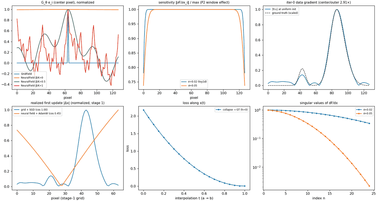
toy1d (n = 128): filter-kernel rows of a grid vs a neural field at three annealing levels; sensitivity for two blur widths; the iter-0 data gradient; realized first updates; the loss along a straight path; singular-value decay for two blur widths.

diagnostic	measures	paper reference	nefi on toy1d / NV
`sensitivity_map`	`‖∂F/∂x_i‖` per pixel	NeTMY Eq. 23, (P2)	edge pixels 22–26 % less visible (toy)
`iter0_gradient`	`∇ₓL` at a uniform init + center/outer ratio	NeTMY §5.3: 18.29×, peak at center	NV 64², F2: 14.3× (peak r = 0.13); F1: 0.24×
`energy_barrier`	loss along `(1−t)x_a + t x_b`	NeTMY Fig. 4b: h ≈ 1.12 at t = 0.20 (F2)	0 for convex toy losses
`center_mass_ratio`	mass in a central disk	NeTMY Fig. 4c: 0.00 … 0.223	uniform baseline 0.071 (2-D)
`filter_kernel_row`	row of `G_θ = J_θ J_θᵀ`	NeTMY Lemma 2, Eq. 32–39	grid 1 px; neural 128 → 21 → 7 px (β/K = 0, ½, 1)
`realized_update`	`\|Δx\|` after 1 step vs `\|∇ₓL\|`	NeTMY App. E.5: 1.6× vs 18.29×	grid+SGD: cos 1.000, damping 1.000
`effective_bandwidth`	highest active Fourier band	NeTMY Eq. 37	0 → 2 → 16 cycles (toy, K = 6)
`singular_values`	top-k σ of `dF/dx`	NeFTY Prop. 2 (`σ_n ≲ n^(-1/3)`), NeTMY Lemma 1	σ₂₄/σ₁ = 0.34 (σ = 0.02) vs 0.0022 (σ = 0.05)
`hessian_condition_number`	`κ(∇²L)` on a small ansatz	NeTMY Fig. 5: κ_F2 = 931, κ_F1 = 301,139	—
`data_fit_paradox`	data PSNR next to field metrics	NeFTY App. G.2: PINN 63 dB surface at IoU 0.01	toy: 38 dB data, 28 dB field, RMSE/σ ≈ 1.2

Sensitivity: what does the instrument see?¶

s = D.sensitivity_map(problem)                      # Hutchinson-style estimate, 32 probes
s_exact = D.sensitivity_map(problem, exact=True)    # one JVP per pixel (small grids)
D.center_to_outer_ratio(s)                          # mean |s| in a central disk / outer ring

The column norm ‖∂F/∂x_i‖ = sqrt((JᵀJ)_ii) says how strongly pixel i influences the measurement (NeTMY Eq. 23). Estimators: method="output" (default) averages (Jᵀu)² over Rademacher probes u in measurement space — reverse-mode only, non-negative, with a relative error ≈ sqrt(2/n_probes) independent of the operator's blur width; method="hutchinson" averages v ⊙ JᵀJ v (jvp then vjp) over field-space probes; exact=True computes every column.

Read it as:

window center bias (P2) — on a finite window, the footprint of an edge pixel is truncated, so edge pixels are less visible and the raw data gradient points toward the center (panel 2: the wider the blur, the wider the low-sensitivity border);
depth decay — in heat conduction the sensitivity of deep voxels is orders of magnitude below the surface (on the thermal_tomography smoke problem nefi measures a max/min ratio of ≈ 280), the pointwise counterpart of NeFTY App. B.4;
a trust mask — report low-confidence where s is small (NeFTY's limitations section asks for exactly this); combine with seed ensembles (nefi.solve.ensemble).

Pass fields= to linearize at another point (e.g. the ground truth or a result) and field= to differentiate with respect to another field.

The iteration-0 gradient: what does a free-pixel solver do first?¶

g = D.field_gradient(problem, fields=None, terms="data")   # raw ∇ₓL at any field values
sig = D.iter0_gradient(problem)                            # at a uniform initialization
sig.ratio, sig.peak_index, sig.peak_radius, sig.center_mass

A free-density solver (Tikhonov, ADMM, a GridField) executes ∇ₓL verbatim. NeTMY §5.3 shows that under the physically faithful operator F2 the very first gradient already peaks at the grid center with a center/outer ratio of 18.29× — before any structure has formed — because the window bias (P2) and the max-normalization peak coupling of the log-MSE (P3, Eq. 24) compound. nefi reproduces the signature on the nv_relaxometry instance at the paper resolution (64², scene many/close, seed 0):

inversion operator	iter-0 center/outer ratio	peak location
F2 (tensor, physical)	14.3×	r = 0.13 (near the center)
F1 (scalar, coherent)	0.24×	r = 1.35 (a corner)

A large ratio with a central peak predicts centered collapse for free-pixel solvers; the remedy is a parameterization that does not execute this gradient verbatim (below), restarts, or a mean-normalized fidelity (NormalizedMSE("mean"), NeTMY's R_nm).

center_mass_ratio(x, radius_fraction=0.15) is the fraction of Σ|x| inside a central disk of diameter 30 % of the side. Compare with uniform_center_mass(shape) (0.071 in 2-D, 0.30 in 1-D): NeTMY reports 0.00 (NeTMY) < 0.064 < 0.081 < 0.153 < 0.223 (Tikhonov) after 200 iterations, and an ADMM aggregate rising from 0.55 to 0.78 from F1 to F2.

Energy barrier: can descent escape?¶

eb = D.energy_barrier(problem, fields_a=collapsed, fields_b=gt, n=21)
eb.height, eb.t_max, eb.monotone, eb.loss          # NeTMY F2: h ≈ 1.12 at t = 0.20

The loss along the straight line from a state a (e.g. a centrally collapsed iterate of a grid solver) to b (the ground truth). A positive height = max_t L(t) − L(0) means a gradient method sitting at a must climb to move toward the truth along this path; NeTMY finds h ≈ 1.12 under F2 and a monotone profile under F1. For a convex loss (linear operator + MSE + TV, panel 5) the height is always 0. To reproduce Fig. 4b you need a collapsed iterate: run a free-pixel baseline (inst.baselines()["grid"]) and check center_mass_ratio of its result first — at a 200-step budget nefi's Tikhonov baseline on NV many/close reaches only 0.093 (uniform: 0.069), i.e. it has not collapsed yet and shows no barrier; the barrier is a property of the collapse basin.

The filtering view: `G_θ = J_θ J_θᵀ`¶

row = D.filter_kernel_row(problem, pixel="center", progress=1.0)   # G_θ e_i, field-shaped
D.kernel_spread(row)                                               # main-lobe half-max width (px)

A gradient step on the parameters θ of a field x = f_θ changes the field by (NeTMY Lemma 2)

Δx ≈ −η J_θ J_θᵀ ∇ₓL = −η G_θ ∇ₓL

so the realized update is the raw gradient filtered by the positive semidefinite kernel G_θ. filter_kernel_row computes one row matrix-free — a VJP (J_θᵀ e_i, one backward pass) followed by a JVP through the field module. For a GridField the row is a delta (G_θ = I, width 1 px): the raw gradient, including the center bias, is executed verbatim. For a NeuralField it is a smooth, spatially coupled kernel whose width shrinks as the annealing opens higher Fourier bands (panel 1: 128 → 21 → 7 px at β/K = 0, ½, 1 on toy1d) — the low-pass behaviour of Eq. 38–39 at small β, and the reason a sharp center spike in ∇ₓL is not executed as a singular update. D.effective_bandwidth(field, progress) reports the highest active band B_β (Eq. 37).

Realized update vs raw gradient¶

ru = D.realized_update(problem)                 # one real optimizer step on a copy of the field
ru.delta_ratio, ru.grad_ratio, ru.damping, ru.alignment
D.realized_update(grid_problem, optimizer="sgd")   # Lemma 2 setting: vanilla step

The field module is deep-copied and stepped once exactly as the solver would (stage resolution, loss weights, learning rate and annealing progress at step 0, the curriculum's optimizer, gradient clipping); the step is taken in float64 so the tiny update is not lost to rounding. alignment is the cosine between Δx and −∇ₓL, damping the ratio of the center/outer ratios. Reference points: NeTMY App. E.5 measures a realized ratio of 1.6× against 18.29× for the raw gradient (≈ 11× damping). In nefi, a grid with SGD gives alignment = 1.000, damping = 1.000 (verbatim, as Lemma 2 predicts); the toy neural field gives alignment = 0.45 and damping 15.9. The markdown report also prints the paper-style damping (iter-0 data-gradient ratio ÷ realized ratio).

Singular values: how ill-posed is it?¶

sv = D.singular_values(problem, k=24, n_iter=60)                  # non-increasing, float64
sv, vecs = D.singular_values(problem, k=8, return_vectors=True)   # right singular vectors

Lanczos with full reorthogonalization on JᵀJ, each product a JVP then a VJP — matrix-free, so it works for 3-D PDE operators. The decay of σ_n is the operator-theoretic statement of ill-posedness: NeFTY Prop. 2 proves σ_n ≲ n^(-1/3) for the linearized heat map on a slab (and Cor. 1: the pseudo-inverse amplifies noise along the n-th mode by 1/σ_n); NeTMY Lemma 1 bounds the dipolar kernel's spectrum by e^(-k z0). Panel 6: tripling the blur width moves σ₂₄/σ₁ from 0.34 to 0.0022. The right singular vectors show which field patterns the measurement can see (the rest must come from the prior). On toy1d the top singular value matches max |FFT(kernel)| = 1 to 0.2 %, and all top values match a dense SVD to 1e-3 (tests/test_diagnostics.py).

Hessian conditioning on an ansatz¶

def gaussian(p, r):                       # ρ(r; A, σ) = A exp(−‖r − c‖²/2σ²), p = (log10 A, σ)
    return 10 ** p[0] * torch.exp(-((r - 0.5) ** 2).sum(-1) / (2 * p[1] ** 2))

fn = D.ansatz_objective(problem, gaussian)          # loss as a function of 2 numbers
kappa = D.hessian_condition_number(fn, [0.0, 0.1])  # at a minimum of fn
evals, H = D.hessian_spectrum(fn, [0.0, 0.1])

NeTMY App. E.8 evaluates the log-MSE on the α-RuCl3 data with a Gaussian density ansatz and finds κ_F2 = 931 (a parabolic bowl) vs κ_F1 = 301,139 (a degenerate valley along A²σ² = const, because Γ ∝ A² under F1). Use it to compare operators or losses on a physically meaningful low-dimensional slice. Evaluate at a minimum (an indefinite Hessian is flagged) and use float64 (problem.to(dtype=torch.float64)) for large κ.

The data-fit paradox¶

fit = D.data_fit_paradox(result, problem, gt)
fit["data_psnr"], fit["field_psnr"], fit["discrepancy_ratio"]

NeFTY App. G.2: the soft-constrained PINN fits the surface thermograms at ≈ 63 dB while its volumetric IoU is 0.01 — a good data fit does not imply a correct field when the forward map is strongly smoothing. Always report measurement-space fit next to field-space metrics. discrepancy_ratio = RMSE / σ (when the noise level is known) should approach 1 (Morozov); well below 1 means the solver fits noise — use Curriculum(discrepancy_tau=1.0) to stop there.

Pathology → signature → diagnostic → remedy¶

pathology	signature	diagnostic	remedies in nefi
(P1) frequency suppression	fast singular-value decay; fine detail unrecoverable	`singular_values`, `sensitivity_map`	annealed `FourierFeatures`, multiscale `Curriculum`, TV / Laplacian priors
(P2) window center bias	edge pixels less visible; centered raw gradient	`sensitivity_map`, `iter0_gradient`	neural field (`G_θ` smoothing), restarts, padding the domain
(P3) max-normalization coupling	peak self-reinforcement, energy barrier	`iter0_gradient`, `energy_barrier`, `center_mass_ratio`	`NormalizedMSE("mean")` companion, gated heads, annealing
(P4) merging / joint ambiguity	cross artifacts, arbitrary background parameters	`filter_kernel_row`, `singular_values` (right vectors)	`SupportMasked` heads, `Laplacian` / isotropic TV, FAQ
soft-constraint decoupling	high data PSNR, near-constant field	`data_fit_paradox`	hard physics (an `Operator`, never a residual penalty)
inverse crime	optimistic benchmarks	`bench.check_inverse_crime`	independent `DataGenerator` (tutorial 3)

Plots¶

nefi.diagnostics.plots (matplotlib optional, pyplot-free so it is safe on servers): plot_report(report), plot_sensitivity, plot_filter_kernels, plot_energy_barrier, plot_singular_values, plot_history, plot_result, show_field (1-D line, 2-D image, 3-D mid slice) and save_figure(fig, path).

Cost¶

diagnostic	operator calls
`sensitivity_map`	1 forward + `n_probes` VJPs (Hutchinson: + `n_probes` JVPs); exact: 1 JVP per pixel
`singular_values`	`n_iter` × (JVP + VJP)
`iter0_gradient`, `field_gradient`	1 forward + 1 backward
`energy_barrier`	`n` forwards
`realized_update`	2 forwards + 1 backward
`filter_kernel_row`	no operator call (field only)

JVPs use forward-mode AD when the operator supports it; otherwise the double-backward trick; as a last resort central finite differences (with a warning). diagnose() computes the sensitivity exactly up to 1024 pixels and records every failure in report.errors instead of raising.