darcy_flow — permeability from steady pressure data

At a glance
Problem	Log-permeability of a closed reservoir from sparse pressure gauges under several well configurations (hydraulic tomography)
Unknown	Y = log k, 32²
Physics	−∇·(k∇p) = well sources with no-flow boundaries; harmonic-mean finite volumes, PCG, implicit-function-theorem adjoint
Measurement	gauge pressures on an 8 × 8 sensor lattice for 6 injector / producer configurations; data on a 2× grid in float64
Difficulty classes	smooth, channels
Baselines	grid
Metrics	PSNR · SSIM · MSE · relative error · high-permeability IoU
Run	nefi run darcy_flow --smoke · full: nefi run configs/darcy_flow_full.yaml --device cuda

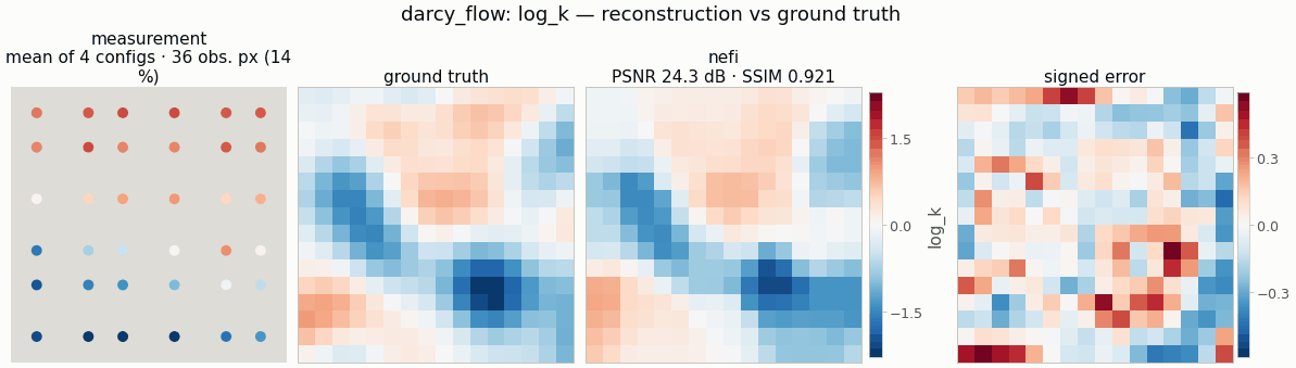
Gallery run (smoke preset: 16², 4 well configurations; 400 steps, 3.9 s on a CPU): PSNR 24.3 dB.

Recover the log-permeability Y = log k of a closed 2-D reservoir from sparse pressure gauges recorded for several injector/producer well configurations (hydraulic tomography / history matching; Bear 1972, Yeh & Liu 2000, Oliver, Reynolds & Liu 2008):

q = −(k/μ)∇p,   ∇·q = f   ⇒   −∇·(k∇p) = μ Σ_w Q_w δ(x − x_w),   no-flow (Neumann) boundary

from nefi.instances.darcy_flow import DarcyFlow
out = DarcyFlow(n=16, n_configs=4, n_sensors=6, steps=(50, 100), lr=1e-2, n_octaves=3).run(seed=0)
out.metrics      # {"psnr", "ssim", "mse", "relative_error", "high_k_iou"}  (on log k)

CLI: nefi run darcy_flow --smoke, nefi run configs/darcy_flow_full.yaml --device cuda. Example: python examples/darcy_flow.py --config configs/darcy_flow_smoke.yaml.

Physics and discretization (nefi.instances.darcy_flow.operator)

• DarcyOperator(domain, wells, sensors=..., obs_shape=...) — an EllipticOperator with sigma_transform="exp" (field log_k), harmonic-mean faces, pure-Neumann Jacobi-PCG (the balanced well rates satisfy the compatibility condition; the solver still projects and pins the mean pressure), implicit-function adjoint, warm starts, one right-hand side per configuration.
• Wells (well_configurations): configuration c has an injector (+Q) at angle θ_c = well_angle + πc/n_configs and a producer (−Q) opposite, at well_radius × L from the centre; point sources are cloud-in-cell spread (point_source_rhs), so the discrete rate is exact and the source moves smoothly with its position at every resolution.
• Sensors (sensor_mask): a regular n_sensors × n_sensors lattice snapped to cells; for each configuration gauges within well_exclusion cells of its wells are dropped (the well-cell pressure has a grid-dependent log singularity and is not a resolution-consistent observable).
• Observable — the pressure solved on the operator's grid is sampled on the native grid (bilinear from coarser curriculum grids, cell averages from finer ones) and referenced to the mean over the gauges (gauge pressure). Coarse stages therefore predict the native sensors directly: at 32² the coarse (16²) model misfit at the true field is 5.6 % of the signal (vs 19 % when the data were instead averaged onto coarse cells).

Data (inverse-crime guard)

Same physics on a 2× finer grid in float64, gauge values = native cell averages, Gaussian noise noise_std × max|p|; fidelity_tag = "elliptic-fv-2x-float64". Scenes (DarcyScenes, closed-form in position so fine and native grids agree):

class	content
smooth	log-normal Y = μ + s·G, G a unit-variance Gaussian random field with squared-exponential covariance of length corr_length (random Fourier features)
channels	weaker background (channel_bg_std) + 1–3 sinuous high-permeability channels (+channel_contrast in Y)

channel_width must span ≥ 2 native cells (smoke: 0.12–0.16 at 16²; full: 0.05–0.08 at 64²).

Inversion

NeuralField (ReLU, few octaves) with Bounded(log_k_min, log_k_max) head → k = exp(Y); masked MSE + isotropic TV(Y); two-stage curriculum (n/2 → n if n/2 ≥ 12, else both at n); baseline grid.

Metrics

psnr, ssim, mse, relative_error on Y = log k, and high_k_iou: IoU of Y > mean(Y_gt) + 1·std(Y_gt) (the flow paths).

Configuration (DarcyConfig)

field	smoke	full	meaning
n, length	16, 1	64, 1	grid / side length
n_configs, well_radius, well_rate, well_angle	4, 0.3, 1, 0.3	8, 0.3, 1, 0.3	wells
n_sensors, sensor_jitter, sensor_seed, well_exclusion	6, 0, 12345, 1.5	12, 0, 12345, 1.5	gauges
tol, grad_mode, warm_start, check_every	1e-6, ift, true, 1	1e-6, ift, true, 8	PDE solver
viscosity, bc, well_spread, face_mode	1, neumann, linear, harmonic	same	physics
scene, log_k_mean, log_k_std, corr_length	smooth, 0, 0.8, 0.15	channels, 0, 0.8, 0.15	scenes
channel_contrast, channel_bg_std, n_channels, channel_width	2.5, 0.4, (1, 3), (0.12, 0.16)	2.5, 0.4, (1, 3), (0.05, 0.08)	channels
channel_amplitude, channel_wavelength, clip_margin	(0.05, 0.12), (0.4, 0.8), 0.2	same	channel meanders, scene clamp
log_k_min, log_k_max	−3, 4	−3, 4	head bounds
noise_std, supersample	2e-3, 2	2e-3, 2	data
hidden, depth, n_octaves, activation	64, 3, 3, relu	256, 6, 4, relu	field
steps, lr, tv	(50, 100), 1e-2, 1e-5	(1000, 3000), 5e-3, 1e-5	optimization

Smoke result (seed 0, smooth, CPU ≈ 7 s): neural PSNR 20.8 dB / SSIM 0.83 vs uniform 12.8 dB / 0.00; grid 22.0 dB / 0.88. At 32² (6 configurations, 8×8 gauges, 450 steps, mean of both classes): neural PSNR 24.1 dB / SSIM 0.77 / high-k IoU 0.64.