The representation is the prior

Choosing how the unknown is parameterized decides which image-space updates gradient descent can make, how fast each spatial frequency converges, and what the reconstruction can and cannot contain. Each physical system therefore calls for a representation whose geometry matches the unknown and whose spectral filter matches the operator's decay — and when we do not know which, the measurement itself can tell us.

This is the thesis nefi distills from NeTMY and NeFTY, and the reason the library treats the representation as a first-class design axis rather than an implementation detail.

The filtering view

NeTMY, Lemma 2. A first-order step on the parameters, \(\theta \leftarrow \theta - \eta\,\nabla_\theta L(f_\theta)\), realizes to leading order the image-space update

\[ \Delta x \;=\; -\eta\, J_\theta J_\theta^{\top}\, \nabla_x L \;+\; O(\eta^2) \;=\; -\eta\, G_\theta\, \nabla_x L, \qquad J_\theta = \partial f_\theta / \partial \theta . \]

\(G_\theta\) is positive semidefinite: every update is the raw data gradient filtered by the representation. What that filter looks like depends entirely on the parameterization:

representation	\(G_\theta\)	consequence
free grid (GridField)	\(I\)	executes the raw gradient verbatim — center bias, noise at all frequencies
MLP + annealed Fourier features	smooth kernel whose band opens with annealing	low-pass early, detail later
Fourier basis	an ideal projector	a hard bandwidth, nothing above the cutoff
Gaussian splats	low rank, localized	moves primitives, cannot fill dense regions
shapes, layers, level sets	columns concentrated on interfaces	moves boundaries, not pixels
coordinate warp	the inner filter at warped coordinates	local bandwidth: detail where the warp stretches

What it predicts

Center collapse (NeTMY). Under the tensor dipolar operator, the data gradient of a uniform density is strongly peaked at the center of the field of view: nefi's iter0_gradient diagnostic measures a center / outer-ring ratio of 112× at 32² (the paper reports 18.29× on its own geometry), against 0.33× — no center bias — under the scalar F1 operator. A free grid (\(G_\theta = I\)) follows that gradient into a collapsed solution; the neural field's kernel spreads the update and escapes it. Diagnostics reproduces the analysis for any problem.

Interior blindness of soft constraints (NeFTY). The heat equation's singular values decay algebraically (Prop. 2), so the surface data constrain the interior only through a hard, exactly solved PDE. With the physics as a soft residual, a network can fit the surface while leaving the interior untouched; with the physics as a hard constraint the only freedom left is the representation — a bounded field with TV, whose filter favours compact, piecewise-constant defects.

Per-frequency convergence. Linearizing around the solution of a translation-invariant problem with operator sensitivity \(\sigma_F(\nu)\) and representation transfer \(g(\nu)\), the error at frequency \(\nu\) evolves as

\[ \hat e_{t+1}(\nu) \;\approx\; \big(1 - \eta\, g(\nu)\, \sigma_F(\nu)^2\big)\, \hat e_t(\nu). \]

A representation is matched when its pass band coincides with the band the data resolve above the noise, over-bandlimited when it cannot express what the data resolve, and under-bandlimited when it moves frequencies the data do not constrain (and fits noise unless annealing, TV or early stopping stops it).

Measuring it

nefi.fields.adaptive.match_report(field, problem) measures both sides — \(g\) from rows \(G_\theta e_i\), \(\sigma_F\) from rows \(J^\top J e_i\) — and states the verdict in words. select_representation lets held-out entries of the measurement choose among candidates.

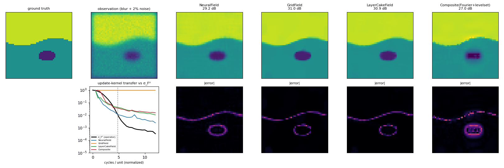
A defect in a two-layer medium (Gaussian blur, 2 % noise, data on a 2× finer grid), four representations with the same losses and 600 steps (examples/geometric_representations.py). Bottom left: the update-kernel transfer of each representation against the operator's sensitivity σ_F²; the dashed line is the band the data resolve.

representation	parameters	PSNR [dB]	defect IoU	match verdict	held-out val/σ²
NeuralField (6 octaves)	11 777	29.2	0.93	over-bandlimited	2.37
GridField + TV	2 304	31.0	0.97	under-bandlimited	1.15
LayerCakeField (layers ⊕ gated anomaly)	2 926	30.9	0.96	matched	1.01
CompositeField (Fourier background ⊕ level set)	2 946	27.0	0.72	over-bandlimited	1.88

The layered representation is the only one whose pass band matches what the data resolve; it recovers the physical parameters (layer values 1.04 / 0.552 against 1.0 / 0.55) with 2 926 parameters, and held-out cross-validation picks it — it predicts unseen measurement entries at the noise floor. The TV grid is a strong baseline for piecewise-constant images under mild blur, and the report says why: it is under-bandlimited, and TV is what keeps it in check.

In practice

• A decision guide from the geometry of the unknown to a representation, an annealing schedule and regularizers: Geometric representations § 3.
• Adaptive tools — residual- and operator-aware annealing, capacity growth, held-out selection and ensembles: § 4.
• After the fact — a smooth result can be re-represented as a multi-phase level set under the same physics and data: Edge refinement.
• When the representation does not matter much — linear problems with a well-tuned explicit prior: Limitations and caveats.