dot3d — continuous-wave diffuse optical tomography

At a glance
Problem	Continuous-wave diffuse optical tomography: the absorption of a scattering slab from surface reflectance
Unknown	absorption μa(x, y, z) (bounded head), 32 × 32 × 16 voxels over 40 × 40 × 20 mm
Physics	diffusion approximation −∇·(D∇Φ) + μaΦ = S with Robin boundaries; Jacobi-PCG, implicit-function-theorem adjoint
Measurement	top-face reflectance on a 12 × 12 detector grid for 3 × 3 sources, calibrated + 1 % noise; data on a 2× grid in float64
Difficulty classes	single, multi, deep
Baselines	grid, deep_decoder
Metrics	PSNR · SSIM · MSE, plus inclusion IoU, depth error and contrast
Run	nefi run dot3d --smoke · full: nefi run configs/dot3d_full.yaml

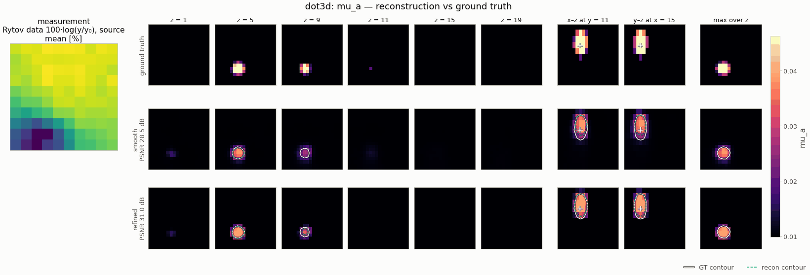
Gallery run (20 × 20 × 10; 700 steps, 17.9 s on a CPU): PSNR 28.5 dB; edge refinement accepted, IoU 0.71 → 0.74. Rotate it in the 3-D showcase.

Recover the absorption coefficient μ_a(x, y, z) (mm⁻¹) of a tissue-like scattering slab (μ_s' = 1 mm⁻¹, background μ_a = 0.01 mm⁻¹) from the diffuse reflectance measured by a camera-like grid of detector pixels on the top face, for 3×3 point sources on the same face. It is the surface-to-volume elliptic inverse problem and NeFTY's structural twin: data on one face only, a strongly smoothing forward map, and a sensitivity that decays by two orders of magnitude with depth.

DOT3DScenes (single | multi | deep inclusions) ─► diffusion FV on a 2× grid (float64), calibrated ─► (9, n_dx, n_dy) + 1 % noise
coords ─► annealed Fourier PE (3-D) ─► ReLU MLP ─► Bounded(0.8 μ_bg, μ_max) ─► μ_a
       ─► −∇·(D∇Φ) + (μ_a + κ_Robin) Φ = S  (Jacobi-PCG, IFT adjoint, warm starts) ─► top-face exitance / reference
       ─► masked relative MSE + λ·TV₃D ─► two-stage multiscale ─► PSNR / SSIM / inclusion IoU / depth error / contrast

from nefi.instances.dot3d import DOT3D

inst = DOT3D(preset="smoke")              # 40×40×20 mm on 20×20×10 voxels, 150 + 200 steps
out = inst.run(seed=0, device="cpu")
print(out.metrics)                        # psnr, ssim, mse, iou, iou_2d, depth_error, depth_rmse, contrast
sens = inst.sensitivity(n_probes=64)      # ‖∂y/∂μ_a(x)‖ at the background (nefi.diagnostics)

CLI: nefi run dot3d --smoke, nefi run configs/dot3d_full.yaml, nefi bench dot3d --smoke --methods neural,grid --classes all. Example: python examples/dot3d.py [--set scene=deep] writes dot3d.png (depth slices and an x-z cut of GT / NF / voxel grid, the calibrated data and the sensitivity maps / depth profile) and metrics.json under runs/dot3d_smoke/.

Physics (nefi.instances.dot3d.operator)

Diffusion approximation of the radiative transfer equation (Arridge, Inverse Problems 15, 1999; Durduran et al., Rep. Prog. Phys. 73, 2010) with the absorption-independent diffusion coefficient D = 1/(3μ_s') (Furutsu & Yamada 1994), known and homogeneous:

−∇·(D∇Φ) + μ_a Φ = S,        Φ + 2AD ∂_nΦ = 0 on every face,       A = (1 + R_eff)/(1 − R_eff)

(R_eff from the Groenhuis fit of the refractive-index mismatch, A ≈ 3.25 at n = 1.4; Haskell et al. 1994). Sources: isotropic point sources one transport mean free path 1/μ_s' below the top face (cloud-in-cell, re-derived at every resolution). DiffuseOpticalOperator subclasses nefi.physics.elliptic.EllipticOperator (cell-centered finite volumes, harmonic faces, Jacobi-PCG, implicit-function adjoint, warm starts) and overrides three hooks:

• coefficient() — the known D on the grid (the field provides only μ_a);
• kappa_value() — κ = μ_a + κ_b: the exact finite-volume Robin flux as Neumann sides plus a boundary-cell sink κ_b = K_b/h, K_b = 1/(2A + h/2D) (the half-cell diffusion resistance in series with the boundary "film"); no ghost state, second order;
• post() — the top-face exitance J = K_b Φ₀, bilinearly interpolated and averaged over each detector's square footprint (3×3 sub-samples), then calibrated by the readings of the homogeneous reference slab (reference_mua, solved once per resolution/device/dtype and cached): the normalized data of difference DOT (O'Leary et al. 1995; Pogue et al. 1999). Unknown source / detector couplings and most of the systematic discretization error cancel in the ratio.

The output (n_sources, n_dx, n_dy) does not depend on the grid, so every curriculum stage fits the same measurement. The map is monotone (more absorption, less light) and not homogeneous (homogeneity = None).

Data, scenes, losses

DOT3DScenes (physical mm, cell-averaged spheres of raised absorption): single (one inclusion, center depth 5–8 mm), multi (2–3 laterally separated inclusions at 4–11 mm), deep (one at 10–13 mm), radius 3–5 mm, μ_a 0.03–0.05 mm⁻¹ (3–5× the background). DOTDataGenerator simulates on a 2× finer grid in float64 (fidelity_tag = "dot-fv-robin-2x-float64" vs "dot-fv-robin-calibrated"), masks source–detector pairs closer than min_separation = 6 mm (diffusion theory fails there and they dominate the dynamic range) and applies 1 % multiplicative Gaussian noise (per-entry noise_std tensor). Data term: RelativeResidualMSE — mean_obs [(pred − obs)/|obs|]², the weighted least squares of multiplicative noise; prior: isotropic 3-D TV (tv = 1).

The head Bounded(μ_min = 0.008, μ_max = 0.1) starts at the background; with μ_min just below μ_bg the sigmoid's flat lower tail acts as an absorbers-only prior (inclusions add absorption). It is the single most effective setting found: with μ_min = 0.002 the half-max IoU of a single- inclusion scene drops from 0.83 to 0.58 and the depth error rises from 0.5 to 1.2 mm (24×24×12 slab, TV 1, tanh field). TV had to be raised to 1: at 1e-2 it is ~100× weaker than the data term and the deep, unconstrained voxels drift (half-max IoU 0.24 at TV 0.1 vs 0.58 at TV 1, same setting).

Sensitivity: why depth is hard (nefi.diagnostics.sensitivity_map)

sens = inst.sensitivity(n_probes=64)       # column norms of the Jacobian at μ_a = μ_bg (masked data)
profile = sens.mean(dim=(0, 1))            # per depth slice

DOT3D.sensitivity() linearizes the calibrated operator at the homogeneous background and returns ‖∂y/∂μ_a(x)‖ (stochastic output probes, i.e. one adjoint solve per probe; exact=True costs one solve per voxel). On the smoke slab (2 mm voxels) the mean sensitivity falls ≈ 200× from the top to the bottom slice (205× with exact columns, 160× with the 64-probe estimate), monotonically, and laterally it peaks under the sources: the data barely constrain the lower half of the slab. This is the reason for the depth metrics below, for the depth-dependent contrast loss of every method, and for the deep class. tests/test_dot3d.py asserts a > 10× top/bottom ratio and a monotone profile.

nefi diagnose dot3d --smoke runs the whole diagnostics report on this operator (≈ 2 s): the sensitivity dynamic range is 1.4e5 (max/min over the voxels), the top singular values of dF/dμ_a are 100, 57.5, 57.3, 44.2, and the neural-field filter kernel G_θ e_i has a 16-voxel main lobe at β = 0 (13 at β = K). The Jacobian-vector products behind these numbers are exact in every mode: forward mode (torch.func.jvp, the diagnostics' default) uses the implicit-function tangent rule of the elliptic core (u̇ = A⁻¹(ḃ − (∂A/∂σ·σ̇)u − κ̇⊙u), one cold-started PCG solve, so warm starts cannot truncate tangents), and double backward / Hessian-vector products work because the detector readout is an index gather (twice differentiable, unlike grid_sample). The top singular values agree across jvp_mode = forward / double_backward to 5e-5 (float32). The operator keeps no torch.func wrapper in its caches (the calibration reference is solved on the transform-safe implicit path when first requested inside a transform, and not cached then).

Metrics (DOT3D.evaluate)

Contrast-independent, because DOT under-recovers the absorption contrast by design (the smoothing forward map spreads a compact inclusion over a larger, weaker blob):

• psnr, ssim (slice-averaged), mse on μ_a;
• iou — volumetric IoU of the half-maximum masks {e > ½ max e} of the absorption excess e = [μ_a − μ_bg]_+ (iou_fraction), iou_2d — the lateral footprint IoU;
• depth_error — |z̄_pred − z̄_gt| (mm) of the excess-weighted inclusion centroids;
• depth_rmse — RMSE (mm) of the 2.5-D excess-weighted depth maps over the columns detected in both (NeFTY App. H-style; NaN if none);
• contrast — recovered / true peak excess (1 = full contrast recovery).

Configuration (DOT3DConfig) and presets

field	default	smoke	meaning
extent, grid	(40, 40, 20) mm, (32, 32, 16)	(20, 20, 10)	slab, voxels (last axis = depth)
musp, refractive_index, mua_background	1.0, 1.4, 0.01		optics (mm⁻¹)
source_grid, source_span	(3, 3), 0.6		sources on the top face
detector_grid, detector_span, detector_samples	(12, 12), 0.85, 3	(10, 10)	detector pixels
min_separation, calibrate, noise_std, supersample	6 mm, true, 0.01, 2		data
tol, max_iter, check_every, warm_start	1e-7, null, 1, true		PCG (float32 floor ≈ 1e-6)
scene, inclusion_mua, inclusion_radius, depth_*, lateral_span	single, (0.03, 0.05), (3, 5), …		scenes
mua_min, mua_max, log_param	0.008, 0.1, false		head (LogBounded if log_param)
hidden, depth, skip_at, n_octaves, activation	128, 4, 2, 4, relu	64, 3, 2	neural field (ReLU, as NeFTY)
tv, tv_eps	1.0, 1e-4		TV weight
steps, lr, lr_decay, anneal_fraction, min_coarse	(300, 600), 1e-2, 0.5, 0.3, 6	(150, 200)	curriculum
iou_fraction, grid_lr, dd_*	0.5, 5e-2, …		metrics / baselines

Presets: smoke, multi, deep, default. Configs: configs/dot3d_smoke.yaml, configs/dot3d_full.yaml (32×32×16, 600 + 1200 steps).

Baselines (DOT3D.baselines())

grid (free voxels with the same bounded head, TV and calibrated operator) and deep_decoder. There is no closed-form classical reference in the instance; the linearized (Born/Rytov) Tikhonov one-step reconstruction is a natural addition (the Jacobian columns are −Φ_s G_d from one forward and one adjoint solve per source / detector).

Validation (tests/test_dot3d.py, ≈ 25 s)

check	result
exact finite-volume flux balance: absorbed + escaped through the Robin faces = source power	to 1e-8 (1e-6 asserted)
diffuse reflectance vs the semi-infinite dipole solution (Farrell, Patterson & Wilson 1992), 1 mm voxels	ratio 1.02–1.06 at 12–20 mm (1.09–1.14 at 8–10 mm; the dipole's extrapolated boundary is itself approximate near the source)
convergence of the uncalibrated readings vs a 96×96×48 reference	7.6 % (24³-class), 3.0 % (32), 1.1 % (48): second order, large constant from the near-boundary source
calibrated native-vs-2× model mismatch (24×24×12, six scenes)	0.07–0.9 % rms (raw: 6.5 %)
IFT gradient vs central finite differences (float64, tol = 1e-12)	≤ 1e-5 relative
forward-mode (torch.func.jvp) and double-backward JVPs vs central differences (fresh, warm-started operator)	≤ 1e-5 relative
sensitivity top / bottom slice (smoke slab)	205× exact, 160× from 64 probes (> 10× asserted)
scenes: depth classes separated, avg_pool(2× render) = native	≤ 1e-6

Solver cost (one CPU thread, 9 sources batched, warm-started): 20×20×10 forward + adjoint 25 ms (21 / 24 PCG iterations), 32×32×16 98 ms (29 / 30). The CG tolerance must stay tight: with warm starts a relative tolerance of 1e-4 (measured against the source-dominated right-hand side) lets the solver return after 0 iterations while the far-detector readings still lag the field, and the inversion fails (PSNR 2.7 dB).

Inversion (smoke preset, 1 % noise; mean over seeds 0–1; PSNR dB / SSIM / half-max IoU / depth error mm / contrast):

scene	method	PSNR	SSIM	IoU (½ max)	depth error [mm]	contrast	time [s]
single	neural field	26.3	0.905	0.58	0.95	0.63	17
single	voxel grid	25.4	0.896	0.59	1.08	0.48	10
multi	neural field	19.0	0.617	0.28	0.74	0.31	8
multi	voxel grid	19.1	0.632	0.32	0.75	0.28	6
deep	neural field	22.2	0.856	0.24	1.29	0.15	8
deep	voxel grid	22.0	0.845	0.21	1.53	0.12	6

The neural field is at least on par with the free voxel grid under the same objective (the TV + absorbers-only head do much of the regularization work in both) and better where DOT is weakest: contrast recovery and inclusion depth for single and deep inclusions (seed 0 single: NF 28.2 dB, contrast 0.90 vs grid 27.0 dB, 0.64). Every method loses contrast with depth, exactly as the sensitivity profile predicts; times are wall-clock on a 4-thread CPU; the NF smoke run takes ≈ 7 s of CPU time on one core.

Notes and limitations

• Continuous wave only (no frequency or time domain), so absorption and scattering are not separable; μ_s' is assumed known and homogeneous.
• The background μ_a is assumed known (it is the reference of the calibration and the head's starting value); recovering an unknown background needs uncalibrated data or a nuisance scale.
• The inclusions of the multi class at different depths are resolved only partially (the half-maximum masks follow the shallowest, best-sensed one), and the deep class keeps < 20 % contrast — the physics limit shown by the sensitivity map, not an optimizer failure.