current_density — NV-magnetometry current imaging¶
| At a glance | |
|---|---|
| Problem | A thin-film sheet current from the out-of-plane stray field imaged by a widefield NV-diamond magnetometer |
| Unknown | stream function g with K = ∇×(g ẑ), so ∇·K = 0 holds by construction; 64² |
| Physics | planar magnetostatics at a standoff z0: B̂z = (μ0/2) k e−k z0 ĝ, zero-padded FFT |
| Measurement | Bz image + 1 % noise; data by a direct real-space Biot–Savart sum on a 2× grid in float64 |
| Difficulty classes | wires, loops, branching |
| Baselines | grid, fourier (regularized k-space inversion) |
| Metrics | current PSNR · current relative error (+ Bz data-space metrics) |
| Run | nefi run current_density --smoke · full: nefi run configs/current_density_full.yaml |
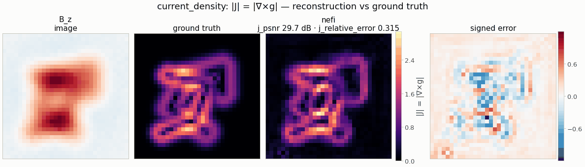
Gallery run (smoke preset: 32², 4-pixel standoff; 600 steps, 0.7 s on a CPU): current PSNR 29.7 dB.
Recover a thin-film sheet current K(x, y) from the out-of-plane stray field B_z measured by a
wide-field NV-diamond microscope at standoff z0 (Roth, Sepulveda & Wikswo 1989; Tetienne et al.
2019; Broadway et al. 2020; Midha et al. 2024 — the static-field sibling of NV noise sensing cited
by NeTMY). The unknown is the stream function g with K = ∇×(g ẑ) = (∂_y g, −∂_x g), so charge
conservation ∇·K = 0 holds by construction:
from nefi.instances.current_density import CurrentDensity
out = CurrentDensity(n=32, pixel=0.25, z0=1.0, steps=(200, 400), lr=1e-2, n_octaves=4, tv=1e-3,
                     hidden=64, depth=3).run(seed=0)                     # the smoke preset
out.metrics      # {"j_psnr", "j_relative_error", "bz_psnr", "bz_relative_error"}
nefi run current_density --smoke, nefi run configs/current_density_smoke.yaml --baseline
fourier. Example: python examples/current_density.py --config configs/current_density_smoke.yaml.
Physics (nefi.physics.magnetostatics)¶
CurrentDensityOperator(domain, z0, mu0, pad_factor=2) — derivation, sign conventions and the
in-plane / NV-axis / sensor-layer variants are in physics_elliptic.md §6.
Units default to μm, mA and μT (μ0 = magnetic_constant("um", "mA", "uT") = 400π). Linear,
homogeneity = 1, rebuilt per curriculum resolution (spacing re-derived, k-grid cached).
Data (inverse-crime guard)¶
BiotSavartDataGenerator with BiotSavartOperator: the scene's g is rendered on a
supersample = 2× finer grid, K is formed with central differences there, and B_z is summed
directly in real space (Biot–Savart midpoint rule, float64, chunked) at the native pixel
centres — no FFT, no padding, no periodic images; fidelity_tag = "biot-savart-direct-float64" vs
"magnetostatics-fft". Noise: noise_std × max|B_z|. The FFT operator at the true g differs
from these data by 1.3–2.7 % (model mismatch). The noise-free field is kept as gt["bz"] for
data-space metrics.
Scenes (CurrentScenes): g = Σ_s I_s Φ(−d_s/w_s) (smoothed indicators; d_s signed distance,
Φ normal CDF) → currents with a Gaussian cross-section of std w_s along region boundaries:
| class | content |
|---|---|
loops |
1–3 elliptical current loops |
wires |
1–2 hairpin circuits (go-and-return wire pairs along a random polyline) |
branching |
trunk + 2–3 branches from a junction with different currents (current splits/merges) |
All sources keep margin from the edges so g → 0 there (no hidden return currents).
Inversion and baselines¶
NeuralField(tanh; ReLU was 2–4 dB worse here) with anIdentityhead forg;RelativeMSEdata term (scale-free in μT) + isotropicTV(g)(piecewise-constantg⇔ currents on thin paths); two-stage curriculumn/2 → n.grid: free pixels + the same losses and curriculum.fourier: the classical regularized k-space inversionfourier_inversion(Tikhonovfourier_regrelative to the transfer peak, Hanning window with cutoffk_c z0 = 3unlessfourier_cutoff), wrapped as aGridFieldinitialized at the reconstruction with a single zero-learning-rate step, so it is reported through the same metrics and benchmark protocol.
Metrics¶
On K = ∇×g (central differences, both components stacked): j_psnr, j_relative_error; on the
predicted field vs the noise-free data: bz_psnr, bz_relative_error.
Configuration (CurrentDensityConfig)¶
| field | smoke | full | meaning |
|---|---|---|---|
n, pixel, z0 |
32, 0.25, 1.0 (4 px) | 128, 0.1, 0.2 (2 px) | pixels, pixel size, standoff (μm) |
length_unit, current_unit, field_unit |
um, mA, uT | same | unit system of μ0 |
nv_layer, pad_factor |
0, 2 | 0, 2 | sensor-layer averaging, FFT padding |
scene, current, width_px, margin |
wires, (0.5, 1.5), (1, 1.5), 0.15 | branching, same | scenes |
loop_radius, wire_separation, branch_width |
(0.08, 0.2), (0.08, 0.14), (0.04, 0.07) | same | scene geometry (fractions of the FOV) |
noise_std, supersample |
0.01, 2 | 0.01, 2 | data |
hidden, depth, n_octaves, activation |
64, 3, 4, tanh | 256, 6, 8, tanh | field |
steps, lr, tv, data_loss |
(200, 400), 1e-2, 1e-3, relative_mse | (1000, 3000), 3e-3, 1e-4, relative_mse | optimization |
fourier_reg, fourier_window, fourier_cutoff |
1e-3, hanning, None | same | Fourier baseline |
Smoke preset = gallery preset: the standoff is 4 pixels (1 μm at 0.25 μm pixels), so the
measured B_z is a smooth, visibly smeared signed map of the thin current paths (at 2 px it looked
like the current itself), and the prior is a piecewise-constant stream function (tv = 1e-3).
Smoke result (seed 0, wires, 600 steps, CPU ≈ 1 s): neural j_psnr 29.7 dB / rel. error 0.32
(seeds 0-3: 28.9-29.7 dB) vs zero field 19.7 dB / 1.0; grid (same objective and budget) 27.9 dB /
0.39; Fourier 21.0 dB / 0.86 — the classical k-space inversion only keeps wavelengths above
2π z0 / 3 ≈ 8 px at this standoff. At a 5 px standoff the neural field still reaches 27-28 dB.
Display (CurrentDensity.viz_hints, nefi.viz.hints): B_z is drawn with a diverging map centred
at 0 and the ground-truth / reconstruction panels show the sheet-current magnitude
|K| = |∇×(g ẑ)|, the quantity the j_* metrics score.