`wave_fwi` — acoustic full-waveform inversion¶

At a glance
Problem	Acoustic full-waveform inversion: a 2-D sound-speed map from the pressure traces of point sources
Unknown	sound speed c(x, z) ∈ [c_min, c_max] (km/s)
Physics	p_tt = c²Δp + s: leapfrog with a 4th-order Laplacian and a PML; gradients through the unrolled scheme or block checkpointing
Measurement	traces (sources × receivers × time) of Ricker sources; surround, transmission or reflection acquisition with a near-offset mute; data on a 2× grid in float64
Difficulty classes	`smooth_anomaly`, `layered`, `scatterers`
Baselines	`grid`
Metrics	PSNR · SSIM · relative error · anomaly error
Run	`nefi run wave_fwi --smoke` · full: `nefi run configs/wave_fwi_full.yaml --device cuda`

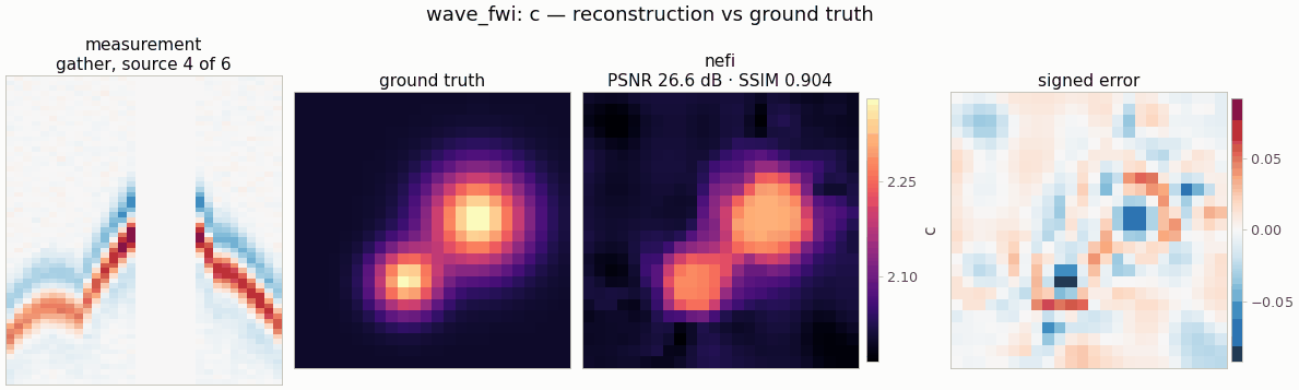
Gallery run (24², 6 sources × 32 receivers; 400 steps, 14.4 s on a CPU): PSNR 26.6 dB.

Recover a 2-D sound-speed map c(x, z) (km/s) on [0, L]² km from pressure traces generated by Ricker point sources:

p_tt = c(x)² Δp + Σ_s w(t) δ(x − x_s),     data d[s, r, j] = p_s(x_r, j·dt_obs) + noise

from nefi.instances.wave_fwi import WaveFWI
inst = WaveFWI(scene="layered", geometry="reflection")        # defaults = CPU smoke preset
out = inst.run(seed=0)                                        # generate -> invert -> evaluate
out.metrics                    # {"psnr", "ssim", "relative_error", "anomaly_error"}

CLI: nefi run wave_fwi --smoke, nefi run configs/wave_fwi_full.yaml, nefi bench configs/wave_fwi_full.yaml --methods neural,grid. Example: python examples/wave_fwi.py [--config ...] [--set scene=layered] (PNG + metrics in runs/wave_fwi_smoke/).

Physics and discretization¶

Operator — nefi.physics.wave.WaveOperator: leapfrog, 4th-order Laplacian, second-order PML (Grote & Sim 2010) of physical width absorb_width, multilinear source/receiver stencils, all sources simulated as one batch. Traces are sampled at fixed times t_j = j·dt_obs; the internal step dt = dt_obs/m obeys the CFL bound for c_max at every curriculum resolution, so the data shape (n_sources, n_receivers, n_t) never changes. Gradients: autodiff through the unrolled scheme (grad_mode="autograd") or block-checkpointed ("checkpoint", memory ∝ √n_steps) — see docs/physics_wave_optics.md §1.
Acquisition — transmission (cross-well: sources at x = margin, receivers at x = L − margin, both spread along depth), reflection (surface: sources and receivers along z = margin), surround (both evenly spaced on the square perimeter; the default).
Near-offset mute — min_offset (km): traces of source–receiver pairs closer than this are zeroed and masked out of the misfit (Measurement.mask, WaveFWI.offset_mask, TraceDataGenerator). Next to a point source the direct wave is dominated by the near field, which the inversion grid and the 2×-finer data grid represent differently: with the unmuted surround smoke acquisition the relative misfit at the true model is 0.049 against 0.077 for the uniform starting model (the modeling error is most of the signal the inversion sees, and it is fitted with artifacts around the sources and receivers); muting offsets below 0.3 km (≈ 20 % of the traces) brings it to 0.011 against 0.098. The full config keeps every trace (min_offset: 0).
Data generation (inverse-crime guard) — the same physics on a supersample = 2× finer grid in float64 (different dispersion error, PML discretization and interpolation stencils), relative Gaussian noise (noise_std × max |trace|). Tags: generator wave-leapfrog-o4-2x-float64, inversion operator wave-leapfrog-o4-pml.
Scenes (WaveFWIScenes, analytic): smooth_anomaly (1-2 Gaussian anomalies of ±(0.6-1)·anomaly in a c_background medium), layered (2-3 dipping interfaces with tanh transitions, increasing speed with depth), scatterers (2-4 smooth-edged disks of radius 0.05-0.09 L).

Prior, objective, curriculum — and cycle skipping¶

Neural field (tanh MLP, annealed Fourier features, Bounded(c_min, c_max) head started at the known background c_background). Losses: fit = relative trace MSE, fit_lo = the same after a zero-phase low-pass (f_low, cosine roll-off, BandLimitedMSE), tv = isotropic TV.

FWI with the L2 misfit suffers from cycle skipping: when the starting model predicts an arrival more than half a period off, gradient descent locks onto the wrong cycle. The default curriculum implements the classic remedy (frequency continuation, Bunks et al. 1995) with Stage.loss_weights:

stage	grid	loss weights	purpose
`low`	`n/2`	`fit_lo = 1`, `fit = 0`	long periods → wide basin; coarse grid resolves them
`full`	`n`	`fit = 1`, `fit_lo = 0`	full band, full resolution

The neural field adds model-space continuation: the annealed Fourier features release high spatial frequencies progressively (NeTMY Eq. 27), and the implicit filtering of the MLP (G_θ = J_θJ_θᵀ) smooths the raw FWI gradient (which is dominated by near-source / near-receiver sensitivity) — the free-pixel grid baseline, with the identical objective and curriculum, lacks both. Set multiscale_frequency: false to ablate the frequency continuation.

Configuration (`WaveFWIConfig`, defaults = smoke preset)¶

field	default	meaning
`n`, `extent`	24, 1.0	grid size, domain side (km)
`scene`	`smooth_anomaly`	`smooth_anomaly` \| `layered` \| `scatterers`
`c_background`, `c_min`, `c_max`	2.0, 1.5, 2.5	km/s; `c_max` is also the CFL bound
`anomaly`	0.4	km/s, anomaly amplitude
`geometry`, `n_sources`, `n_receivers`, `margin`, `min_offset`	surround, 6, 32, 0.08, 0.3 km	acquisition, near-offset mute
`f0`, `t_max`, `dt_obs`	4 Hz, 0.96 s, 0.016 s	Ricker peak, record length, sampling (61 samples)
`order`, `absorbing`, `absorb_width`, `absorb_R`, `courant`	4, pml, 0.25 km, 1e-3, 0.9	solver
`grad_mode`, `checkpoint_every`, `source_batch`	autograd, None, None	memory controls
`noise_std`, `supersample`, `gen_order`	0.005, 2, 4	data generation
`hidden`, `depth`, `n_octaves`, `activation`	64, 4, 3, tanh	neural field
`tv`	1e-3	TV weight
`multiscale_frequency`, `f_low`, `lowpass_taper`, `coarse_factor`	true, 5 Hz, 0.3, 2	curriculum
`steps`, `lr`, `lr_decay`, `grid_lr_mult`	(150, 250), 2e-2, 0.5, 10	optimization

PRESETS["full"] / configs/wave_fwi_full.yaml: 96², 8 sources × 48 receivers (surround, no mute), 8 Hz, 1.2 s at 4 ms (≈ 600 steps), checkpointed adjoint, 256 × 6 MLP, tv 1e-4, 1500 + 3500 steps.

Smoke results (CPU, seed 0, 400 optimization steps = the gallery budget)¶

scene	method	PSNR [dB]	SSIM	anomaly error
smooth_anomaly	initial model	11.3	0.22	1.00
	grid (same objective)	26.1	0.91	0.18
	neural field	26.6	0.90	0.17
layered	initial model	0.6	0.52	1.00
	grid (same objective)	25.2	0.89	0.06
	neural field	25.4	0.86	0.06

(anomaly_error = ‖c − c_gt‖ / ‖c_gt − c_background‖; 1.0 for the starting model; ≈ 12-15 s per neural-field run on a CPU — ≈ 37 ms per 24² step with 6 shots, 1.4× the 2-shot step.) smooth_anomaly over seeds 0-2: anomaly error 0.17 / 0.18 / 0.18 — both anomalies come out as compact blobs at the right place with ≈ 75-80 % of their amplitude (TV flattens the peaks). A transmission acquisition with 2 shots × 8 receivers (100 steps) smears the anomalies into horizontal streaks along the propagation direction — the classic limited-aperture footprint — for PSNR 14.1 dB / anomaly error 0.73; the surround aperture with the near-offset mute removes it, and with that much illumination the free-pixel grid (same objective and curriculum) is on par with the neural field. Small scatterers (1-2 cells, sharp edges) remain harder (anomaly error ≈ 0.5-0.6 on seeds 1-2) — they are near the smoke resolution (λ/2 ≈ 6 cells).

Baselines¶

grid — free-pixel field with the same heads, losses and curriculum (LR × grid_lr_mult). Classical FWI (L-BFGS on pixels) is nefi.baselines.baseline_problem(problem, "lbfgs").

wave_fwi — acoustic full-waveform inversion¶