`holography` — multi-distance inline phase retrieval¶

At a glance
Problem	The phase of a thin transparent sample from inline holograms recorded at several distances
Unknown	phase φ (zero-mean bounded head: the global phase is invisible to intensities), 32²
Physics	thin-object transmission and band-limited angular-spectrum propagation with edge padding
Measurement	intensities at 3 distances + noise; data on a 2× grid in float64, intensities area-averaged onto the pixels
Difficulty classes	`smooth_phase`, `cells`
Baselines	`gerchberg_saxton` (multi-plane), `grid`
Metrics	PSNR · SSIM · RMSE (mean-subtracted)
Run	`nefi run holography --smoke` · full: `nefi run configs/holography_full.yaml`

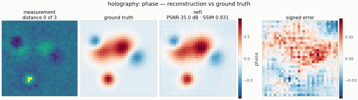
Gallery run (32², 400 steps, 0.6 s on a CPU): PSNR 35.0 dB.

Recover the phase φ(x) (rad) of a thin transparent sample (transmission t = exp(iφ − a) with known constant absorption a, plane-wave illumination) from intensity images recorded at several propagation distances z_i:

I_i(x) = | P_{z_i} t |²(x) + noise,     P_z = angular-spectrum propagator (band-limited)

from nefi.instances.holography import Holography
inst = Holography(scene="cells", distances=(10.0, 25.0, 50.0))
out = inst.run(seed=0)
out.metrics                                   # mean-subtracted {"psnr", "ssim", "rmse"}
gs = inst.gerchberg_saxton(out.measurement)   # multi-plane Gerchberg–Saxton baseline

CLI: nefi run holography --smoke, nefi bench configs/holography_full.yaml --methods neural,gerchberg_saxton,grid. Example: python examples/holography.py.

Physics and discretization¶

Operator — nefi.physics.optics.HolographyOperator: thin-object transmission, zero-phase FFT propagation with the exact transfer function exp(i2πz√(1/λ² − f²)), evanescent waves dropped, Matsushima–Shimobaba band limit, edge padding ×2 (the sample sits in an infinite uniform background; zero padding would add an aperture). Output (n_distances, n, n); the detector pitch equals the field grid spacing at every curriculum stage (coarse stages compare with area-averaged intensities through downsample_obs).
Data generation (inverse-crime guard) — the phantom sampled on a 2× finer grid, propagated in float64 with its own (finer) transfer functions, intensities area-averaged onto the detector pixels (a pixel integrates intensity), then Gaussian noise (noise_std × max intensity). Tags: generator angular-spectrum-2x-float64, inversion angular-spectrum-1x.
Scenes (HolographyScenes): smooth_phase (3-5 Gaussian bumps, ±, normalized to phase_amplitude), cells (2-4 smooth elliptical plateaus with denser nuclei).

Ambiguities and metrics¶

Intensities are invariant to a global phase offset (|P_z(e^{ic} t)|² = |P_z t|²), so the offset is fixed in the model: the phase head is ZeroMean(Bounded(...)) (nefi.fields.ZeroMean, zero_mean = True) — the reconstruction has zero spatial mean by construction — and the phantoms are zero-mean too (HolographyScenes(zero_mean=True); the offset does not change the simulated intensities). Reconstruction and ground truth therefore share one gauge and are directly comparable in every figure; before, the network's arbitrary drift left the reconstruction ≈ 0.5 rad below the truth. The metrics still subtract the mean (phase_psnr, phase_ssim, mean-subtracted RMSE; tested), so they are offset-invariant for any parameterization (zero_mean = False, baselines). A single distance leaves the zeros of the phase-contrast transfer function sin(πλz|f|²) (twin-image / low-frequency ambiguity); several distances (default 10, 25, 50 μm at λ = 0.5 μm, 1 μm pixels) fill them.

Prior, objective and curriculum¶

Neural field with a ZeroMean(Bounded(−phase_bound, phase_bound)) head (default ±π) started at 0, fit = relative intensity MSE, tv = isotropic TV on the phase, two-stage multiscale curriculum n/2 → n.

Configuration (`HolographyConfig`, defaults = smoke preset)¶

field	default	meaning
`n`, `pixel_size`, `wavelength`	32, 1.0 μm, 0.5 μm	detector grid and optics
`distances`	(10, 25, 50) μm	propagation distances
`scene`, `phase_amplitude`, `absorption`	smooth_phase, 1.0 rad, 0.0	phantom
`noise_std`, `supersample`	0.01, 2	data generation
`pad_factor`, `pad_mode`, `band_limit`	2.0, edge, true	propagation
`phase_bound`, `zero_mean`	π, true	head range; `ZeroMean` gauge (and zero-mean phantoms)
`hidden`, `depth`, `n_octaves`	64, 4, 6	neural field
`tv`, `steps`, `lr`, `lr_decay`, `grid_lr_mult`	1e-4, (150, 250), 1e-2, 0.5, 10	objective / optimization
`gs_iterations`	100	Gerchberg–Saxton baseline

PRESETS["full"] / configs/holography_full.yaml: 128² at 0.5 μm, four distances 20-130 μm, 256 × 6 MLP, 1500 + 3500 steps, 300 GS iterations.

Smoke results (CPU, seed 0; mean-subtracted phase)¶

scene	zero phase	Gerchberg–Saxton	grid	neural field
smooth_phase (PSNR / SSIM)	15.9 / 0.02	27.3 / 0.76	31.7 / 0.90	35.0 / 0.93
cells	15.4 / 0.02	28.0 / 0.73	32.9 / 0.88	28.0 / 0.78

(≈ 1 s per neural-field run on a CPU, 400 steps = the gallery budget; smooth_phase over seeds 0-2: 35.0 / 36.0 / 33.3 dB.) The ZeroMean gauge does not change the objective — the fit and TV are offset-invariant, so losses and parameter gradients agree to float32 rounding with and without it — it only removes the arbitrary offset from the reconstruction; metric differences to an unconstrained head are run-to-run (chaotic) variation, up to ±2 dB on cells at this budget. Gerchberg–Saxton leaves a slowly varying phase ramp (the weakly constrained low spatial frequencies); on the piecewise-flat cells the free grid fits the plateaus' sharp edges better than the smooth MLP at this budget.

Baselines¶

grid (free-pixel phase, same objective) and gerchberg_saxton (sequential multi-plane projections with the operator's own propagation model, wrapped as a closed-form "direct" problem).

holography — multi-distance inline phase retrieval¶