`sparse_view_ct` — sparse-view parallel-beam CT¶

At a glance
Problem	Sparse-view (or limited-angle) parallel-beam computed tomography
Unknown	attenuation μ ∈ [0, 1] (bounded head), 64²
Physics	differentiable Radon transform: all views in one `grid_sample`, physical line integrals
Measurement	sinogram of 20 views over 180° + 1 % noise; data on a 2× finer image grid in float64
Difficulty classes	`shepp`, `blobs`, `piecewise`
Baselines	`fbp` (filtered back-projection), `grid` (+ TV), `deep_decoder`
Metrics	PSNR · SSIM · MSE
Run	`nefi run sparse_view_ct --smoke` · full: `nefi run configs/sparse_view_ct_full.yaml`

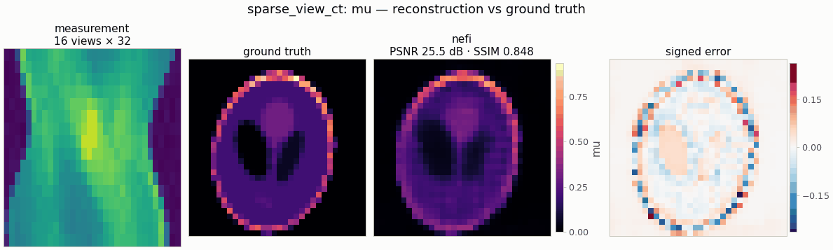
Gallery run (32², 16 views, 450 steps, 0.4 s on a CPU): PSNR 25.5 dB.

Recover an attenuation map μ ∈ [0, 1] on the unit square from n_views (default 20) noisy parallel-beam projections over 180° (or angle_range degrees for limited-angle CT):

y_θ(s) = ∫ μ(s e_θ + t e_θ⊥) dt + n,     θ ∈ {0, π/V, ..., (V−1)π/V}

from nefi.instances.sparse_view_ct import SparseViewCT
inst = SparseViewCT(n=64, n_views=20, scene="piecewise")
out = inst.run(seed=0)
fbp = inst.fbp(out.measurement)          # classical reference on the same sinogram

CLI: nefi run sparse_view_ct --smoke, nefi run configs/sparse_view_ct_full.yaml. Example: python examples/sparse_view_ct.py [--set n_views=12 --set scene=piecewise].

Differentiable Radon transform (`nefi.instances.sparse_view_ct.radon`)¶

RadonOperator(domain, n_views, field="mu", angles=None, angle_range=π, det_per_pixel=1, samples_per_pixel=1) rotates the image with F.grid_sample (bilinear, align_corners=False, zero outside the field of view) for all views at once and sums along the ray direction: p_θ(u_b) = Δt Σ_a μ(R_θ(u_b, v_a)) in normalized coordinates, with Δt the physical ray step, so the sinogram holds physical line integrals. Conventions: axis 1 = x (grid-sample width), axis 0 = y; the detector axis is (cos θ, sin θ); θ = 0 gives column sums. It is linear (homogeneity = 1), batched over leading dims, and at_resolution(shape) keeps det_per_pixel, so n_det scales with the curriculum grid (coarse data are area-averaged over detector bins, which is consistent because each bin is a line integral).

op.adjoint(y) — exact adjoint of this discretization (autograd VJP).
backproject(y, angles, n, width) / op.backproject(y) — classical pixel-driven back-projector (1-D linear interpolation at u = x cos θ + y sin θ), an independent discretization of Rᵀ scaled by Δt · n_t n_det / n².
fbp(sinogram, angles, filter="ramp", n=None, width=1.0, circle=False) / op.fbp(...) — filtered back-projection (π/V) Σ_θ q_θ(x cos θ + y sin θ), q = (h ⊛ p)/τ with the Kak & Slaney discrete ramp h (Kak & Slaney 1988, Eq. 61-62), zero-padded to ≥ 2 n_det, and optional shepp-logan / cosine / hann apodization.

Device note: PyTorch has no MPS kernel for grid_sampler_2d_backward; use CPU or CUDA (MPS is never auto-selected; PYTORCH_ENABLE_MPS_FALLBACK=1 also works).

Data generation and scenes¶

Inverse-crime guard: the data generator uses the same Radon physics on a 2× finer image grid with 2 detector bins per fine pixel (4 sub-bins per native bin) in float64, area-averages the sinogram onto the native detector and adds relative Gaussian noise (fidelity_tag = "radon-2x-float64"; the inversion operator is tagged "radon-<n>px-1det-1spp"). Scenes (CTScenes, inside the inscribed circle, cell-averaged): shepp (modified Shepp-Logan table with random global scale/rotation/shift and random per-ellipse axes, centers, angles, intensities), blobs (smooth Gaussian sums), piecewise (random constant ellipses/rectangles painted in a body ellipse — sharp edges where TV pays off).

Prior, objective and curriculum¶

Neural field with a Bounded(0, 1) head (NeFTY Eq. 6; softplus optional), MSE on the sinogram, isotropic TV (NeFTY Eq. 22) and optional ℓ1, two-stage multiscale curriculum (NeTMY Tab. 6). TV weights are much smaller than in deconvolution because the sinogram MSE at the noise level is ~1e-5 while TV of an edge in physical-gradient units is O(1-10): tv = 1e-5 (sweep: 5e-4 → 18.0 dB, 1e-4 → 21.5, 2e-5 → 26.6, 1e-5 → 28.1 dB / SSIM 0.91, 5e-6 → 28.4 / 0.88).

Configuration (`SparseViewCTConfig`)¶

field	default	meaning
`n`, `extent`	64, 1.0	image size, physical side
`n_views`, `angle_range`	20, 180.0	number of views, angular coverage in degrees
`det_per_pixel`, `samples_per_pixel`	1.0, 1.0	detector bins and ray samples per pixel
`scene`	`shepp`	`shepp` \| `blobs` \| `piecewise`
`noise_std`	0.01	relative Gaussian sinogram noise
`supersample`, `data_det_per_pixel`	2, 2.0	data-generation grid factor and bins per fine pixel
`head`, `init_value`	`bounded`, 0.1	`bounded` (`Bounded(0, 1)`) \| `softplus`
`tv`, `tv_eps`, `l1`	1e-5, 1e-3, 0	regularizers
`hidden`, `depth`, `skip_at`, `n_octaves`, `activation`	128, 4, 2, 7, tanh	neural field
`steps`, `lr`, `lr_decay`, `anneal_fraction`	(400, 800), 1e-2, 0.5, 1.0	curriculum
`fbp_filter`, `fbp_clip`	`ramp`, true	FBP filter; clip FBP to the head range
`grid_lr`	5e-2	grid baseline
`dd_lr`, `dd_width`, `dd_stages`	5e-3, 64, 5	Deep Decoder baseline

Configs: configs/sparse_view_ct_smoke.yaml (32², 16 views, ~4 s CPU), configs/sparse_view_ct_full.yaml (64², 20 views, 1200 + 2400 steps).

Baselines (`SparseViewCT.baselines()`)¶

grid (free pixels + the same TV objective), fbp (closed form through DirectSolver, reported with the same metrics) and deep_decoder. Any other kind is one call away: baseline_problem(inst.build_problem(m), "gaussian_splat" | "admm" | "lbfgs").

Validation¶

tests/test_sparse_view_ct.py (≈ 10 s). Measured values (64², float64):

check	result
`θ = 0` projection vs. column sum × Δt	max abs error 0.0
centered disk (r = 0.25): per-view mass / max variation	1.0e-3 / 5.2e-3 relative; peak chord 0.508 (exact 0.5)
adjoint: `⟨Rx, y⟩` vs `⟨x, backproject(y)⟩`, smooth non-negative fields, 20 draws	≤ 1e-4 relative (30 views), < 5e-5 (180 views); signed fields ≤ 7e-4 of `‖Rx‖‖y‖`
adjoint: autograd `op.adjoint`	1e-15 relative
FBP of a full-view (180) noiseless Shepp-like sinogram	PSNR 25.0 dB (ramp), 24.1 dB (Shepp-Logan)
FBP with 20 views (noiseless)	20.2 dB
linearity `R(2.5a − 0.7b) = 2.5Ra − 0.7Rb`	1e-12

Inversion (seed 0, shepp, 1 % noise; PSNR dB / SSIM):

setting	FBP	neural field	grid + TV	Deep Decoder
32², 16 views, smoke (450 steps)	22.72 / 0.804	25.48 / 0.848 (3.6 s)	27.48 / 0.931 (1.1 s)	27.19 / 0.896
64², 20 views, 300 + 600 steps	21.15 / 0.559	28.39 / 0.919 (34 s)	29.07 / 0.934 (3.8 s)	30.26 / 0.922

All iterative methods remove most of the FBP streaking; with the same TV objective the free grid and the Deep Decoder are at least as good as the neural field in this linear, well-sampled-in- detector setting (single seed; use nefi bench for CIs and per-class results).

Notes and limitations¶

Parallel-beam geometry only (fan/cone beam would need a different sampling grid).
The rotation-based projector is bilinear; for high-accuracy work use det_per_pixel / samples_per_pixel > 1 (costlier) — the data generator already does.
Poisson (photon-count) sinogram noise is not modeled (Gaussian only).

sparse_view_ct — sparse-view parallel-beam CT¶

Differentiable Radon transform (nefi.instances.sparse_view_ct.radon)¶