eit — electrical impedance tomography

At a glance
Problem	Electrical impedance tomography: conductivity from the boundary voltages of injected current patterns
Unknown	σ(x) ∈ [σmin, σmax] (log-parameterized bounded head), 32² on [−1, 1]²
Physics	−∇·(σ∇u) = 0 with Neumann current patterns; harmonic-mean finite volumes, Jacobi-PCG, implicit-function-theorem adjoint
Measurement	boundary potentials of 8 trigonometric current patterns (optional electrode gap model); data on a 2× grid in float64
Difficulty classes	single, multi, contrast
Baselines	grid
Metrics	PSNR · SSIM · MSE · relative error · inclusion IoU
Run	nefi run eit --smoke · full: nefi run configs/eit_full.yaml --device cuda

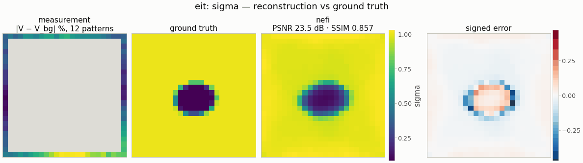
Gallery run (smoke preset: 24², 12 current patterns; 600 steps, 5.3 s on a CPU): PSNR 23.5 dB, inclusion IoU 0.94.

Recover the conductivity σ(x) ∈ [σ_min, σ_max] of a square body [−1, 1]² from the boundary potentials produced by trigonometric current patterns (the Neumann-to-Dirichlet map; Calderón 1980, Cheney, Isaacson & Newell 1999):

−∇·(σ∇u_p) = 0 in Ω,    σ ∂u_p/∂ν = j_p on ∂Ω,    ∮ j_p = 0,    observe u_p|∂Ω,   p = 1..n_patterns
j_{2m} = A cos(2π(m+1)s/P),   j_{2m+1} = A sin(2π(m+1)s/P)        (s = arc length, P = perimeter)

from nefi.instances.eit import EIT
out = EIT(n=24, n_patterns=12, contrast=(8, 12), hidden=128, depth=4, n_octaves=3,
          activation="relu", steps=(200, 400), lr=1e-2).run(seed=0)       # the smoke preset
out.metrics      # {"psnr", "ssim", "mse", "relative_error", "inclusion_iou"}

CLI: nefi run eit --smoke, nefi run configs/eit_full.yaml --device cuda, nefi bench configs/eit_full.yaml --methods neural,grid --classes all. Example: python examples/eit.py --config configs/eit_smoke.yaml → runs/eit_smoke/eit.png.

Physics and discretization (nefi.instances.eit.operator)

• Solver — EITOperator is an EllipticOperator (see physics_elliptic.md): harmonic-mean finite volumes (NeFTY Prop. 1), pure-Neumann Jacobi-PCG with the compatibility projection and zero-mean gauge, implicit-function adjoint, warm starts across optimization steps, all patterns solved as one batch.
• Current injection — eit_boundary(domain, n_patterns, amplitude, electrodes, coverage) walks the boundary faces counter-clockwise from (x_lo, y_lo), assigns each face the face-averaged pattern (so the injected current is exact at every resolution and ∮ j = 0 holds to round-off) and adds j/h_n to the boundary cell's right-hand side (finite-volume flux balance). electrodes = L > 0 switches to the gap model (Somersalo et al. 1992): L electrodes of relative coverage electrode_coverage carry I_l = A (P/L) trig(ω s_l) uniformly, gaps carry nothing, and only electrode cells are observed.
• Observable — for every boundary face the trace u_face = u_cell + (h_n/2) j/σ_cell (second-order extrapolation with the known flux). The traces are mapped by periodic arc-length interpolation onto the faces of the native measurement grid and averaged per strip cell with the observed boundary length as weight; potentials are referenced to their boundary-weighted mean (∮ u = 0 gauge). Every curriculum resolution therefore predicts the same observable, and the measurement is never downsampled. Using cell values instead of traces would leave an O(h) bias of ~65 % of the inclusion signal at 16²; with traces the native model at the true σ reproduces the 2×-finer data to 4 % of the inclusion signal (16²; 3 % at 32²).
• Measurement — (n_patterns, n, n) with mask = boundary strip (or electrode cells); unobserved entries are zero, so no interior potential leaks into the inversion.

Data (inverse-crime guard)

SupersampledObservationGenerator: the same physics on a supersample = 2× finer grid in float64 (tol = 1e-10), observed on the native strip, plus Gaussian noise of noise_std × max|V| on the observed entries; fidelity_tag = "elliptic-fv-2x-float64" vs the inversion's "elliptic-fv". Scenes (EITScenes, analytic ellipses with sub-cell area coverage, background σ_bg = 1):

class	content
single	one conductive or resistive ellipse, contrast 3–6
multi	2–3 non-overlapping ellipses of either polarity
contrast	one ellipse with contrast 10–20 (where the harmonic mean matters most)

Inversion

• field: NeuralField with LogBounded(σ_min, σ_max) head (log_param=True, log-uniform conductivity) or Bounded; ReLU MLP with few Fourier octaves — for this smooth, severely ill-posed problem ReLU was decisively better than tanh (32², 16 patterns, 600 steps: PSNR 23.1 vs 14.8 dB, SSIM 0.87 vs 0.40, inclusion IoU 0.94 vs 0);
• losses: masked MSE + isotropic TV(σ) (tv = 1e-5);
• curriculum: two stages; n/2 → n when n/2 ≥ min_coarse (= 12), otherwise both stages at n (LR decay and annealing restart per stage — in a seeded smoke A/B the restart gained 1.0 dB mean PSNR on EIT, better in 6/6 paired runs, and 0.5 dB on Darcy);
• baseline grid: free pixels with the same head, losses and curriculum (grid_lr).

Metrics

psnr, ssim, mse, relative_error on σ, and inclusion_iou: half-maximum supports (|log σ/σ_bg| > ½ max, each map at its own peak, conductive and resistive matched separately).

Configuration (EITConfig)

field	smoke	full	meaning
n	24	64	cells per axis on [−half_width, half_width]²
n_patterns	12	16	current patterns (frequencies 1…n_patterns/2)
amplitude	1	1	current density amplitude
electrodes, electrode_coverage	0, 0.5	0, 0.5	0 = continuum model
sigma_bg, sigma_min, sigma_max	1, 0.05, 20	same	background and head bounds
contrast, high_contrast, radius, center_radius, inclusion_gap, subsample	(8, 12), (10, 20), (0.2, 0.4), 0.5, 0.1, 4	(3, 6), rest same	scenes
noise_std, supersample	1e-3, 2	1e-3, 2	data
tol, max_iter, precond, grad_mode, warm_start, check_every	1e-6, auto, jacobi, ift, true, 1	same, check_every 8	PDE solver
hidden, depth, skip_at, n_octaves, activation	128, 4, 2, 3, relu	256, 6, 3, 4, relu	field
steps, lr, lr_decay, anneal_fraction	(200, 400), 1e-2, 0.5, 0.5	(1000, 3000), 5e-3, 0.5, 0.5	curriculum
tv, tv_eps, data_loss	1e-5, 1e-3, mse	same	losses
grid_lr	0.05	0.05	grid baseline

Smoke result (seed 0, single — a resistive inclusion, σ ≈ 0.09 in σ_bg = 1 — 600 steps, the gallery's budget at --budget 0.1; ≈ 6 s solve on a CPU, ≈ 10 ms per 24² step): neural PSNR 23.5 dB / SSIM 0.86 / inclusion IoU 0.94 vs uniform 12.3 dB / 0.53 / 0; grid (same objective and budget) 16.7 dB / 0.54 / 0.51. The smoke problem is sized to be informative: with a 16² grid, 4 patterns and 150-200 steps the inclusion comes out as one blurry blob (16.5 dB, IoU 0.46); 8 patterns give 21.3 dB / IoU 0.91, 16 patterns 23.9 dB / 0.91 at 1.3× the step cost. Seed 1 (also resistive) gives 25.6 dB / IoU 0.81. Conductive inclusions of contrast ≈ 10 saturate the boundary data (current already flows through a σ = 3 inclusion almost as through σ = 10): at this budget they are located but blurred and strongly underestimated (seed 2, σ = 10.9: σ_max ≈ 2, IoU 0.39).

Display: the raw patterns are smooth trigonometric profiles around the ring whatever the interior, so the viewers' compact measurement panel (gallery tile, compare figure) shows EIT.difference_data instead (measurement_image hook): per boundary cell, the RMS over the patterns of V − V_bg (V_bg = prediction for the homogeneous body) in % of the RMS boundary voltage — the difference-EIT signature, largest on the side nearest the inclusion (seed 0: 8.6-11.4 %, noise 0.4 %). Full measurement views and data-fit plots stay on the raw stack.