Core concepts¶

nefi solves one kind of problem: an instrument produced a measurement y of a hidden field x through a known physical process F, and there is no paired training data — only this measurement and the physics.

\[ y \;=\; F(x^\star) + \varepsilon, \qquad \hat x \;=\; f_{\hat\theta}, \quad \hat\theta \;=\; \arg\min_\theta \; \mathcal L_{\text{data}}\big(F(f_\theta),\, y\big) + \textstyle\sum_j \lambda_j \mathcal R_j(f_\theta) \]

The unknown is represented by a parameterized field \(f_\theta\) (usually a coordinate neural network), pushed through the differentiable forward model \(F\) at every step, and optimized for this one measurement. Nothing is learned across measurements: every solve starts fresh, which is what makes the method label-free and amortization-free.

The seven pieces¶

piece	what it is	where it lives	the key idea
Domain	a physical box on a cell-centered grid; coordinates normalized to \([-1, 1]^d\)	`nefi.Domain`	the same field can be evaluated at any resolution
Field	the representation \(x = f_\theta(r)\): MLP, grid, hash grid, level set, layered medium, …	`nefi.fields`	the representation is the prior
Heads	value constraints on the raw outputs: softplus, bounded sigmoid, gated, masked	`nefi.fields.heads`	hard knowledge (non-negativity, bounds, support) never needs a penalty
Operator	the physics \(F\): a differentiable map from fields to a prediction of the measurement	`nefi.operators`, `nefi.physics`	a hard constraint, rebuilt at every curriculum resolution
Losses	data fidelity against `y` plus regularizers on the fields	`nefi.losses`	means, not sums: weights do not depend on the grid
Curriculum	stages of resolution, steps, learning rate and frequency annealing	`nefi.solve.Curriculum`	coarse → fine, low → high frequencies
Solver	the optimization loop with its safety features	`nefi.Solver`, `nefi.invert`	per measurement, deterministic, observable

Anatomy of a problem builds each piece by hand; Bring your own problem builds all of them automatically from a forward function.

How a solve proceeds¶

At the start of every curriculum stage the solver rebuilds the coordinates for the stage's grid, asks the operator for its version at that resolution (operator.at_resolution), resamples the measurement consistently, lets the field adapt (a grid resamples itself) and resets the annealing progress \(\beta\). Every step then evaluates field → heads → operator → losses, back-propagates to the field parameters, clips the gradient and takes an optimizer step.

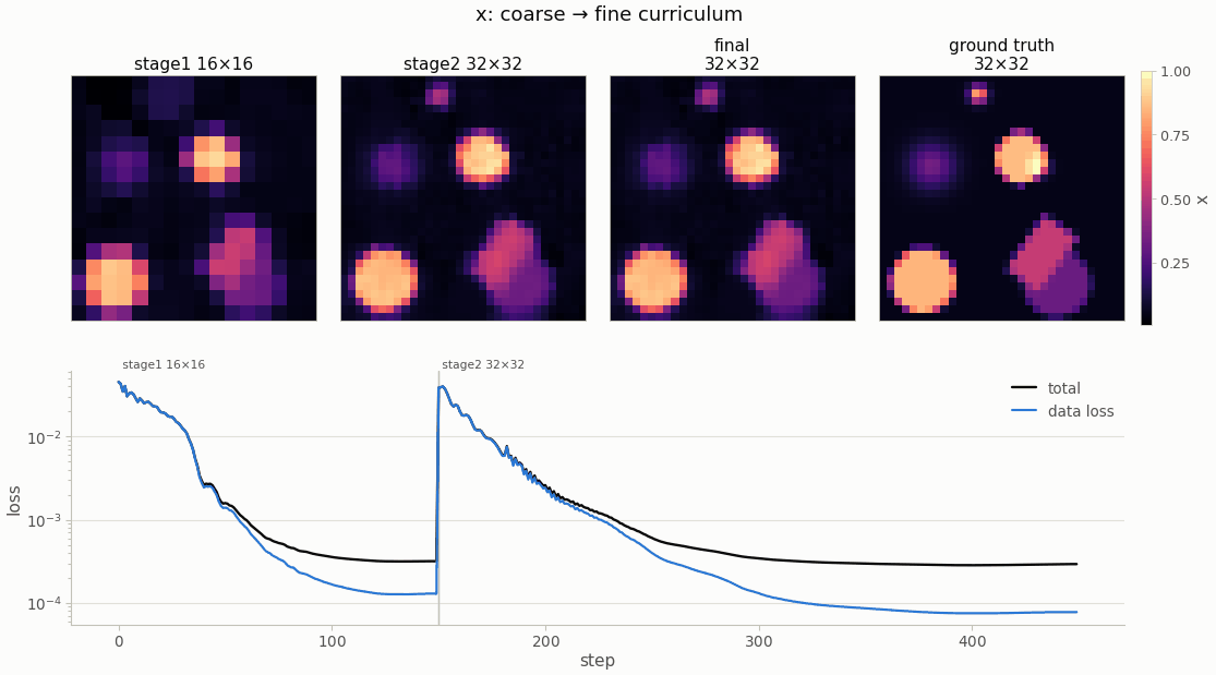
Coarse-to-fine curriculum on the deconvolution instance: the stage-1 result at 16×16, the stage-2 result at 32×32, the final field and the ground truth, with the loss curve of both stages — A two-stage curriculum on `deconvolution` (gallery run, CPU): the coarse stage finds the objects, the fine stage adds the edges; the loss jumps when the resolution and the annealed frequency bands are reset at the stage boundary.

Annealed Fourier features. The encoding multiplies frequency band \(k\) by a weight that rises from 0 to 1 as \(\beta = \text{progress}\cdot K\) passes \(k\) (NeTMY Eq. 27, NeFTY Eq. 21). Early in a stage only low frequencies can change, so the field is smooth; detail is unlocked gradually. The same idea — let the data earn the frequencies — drives the residual- and operator-aware annealing of the geometric representations.

Stopping at the noise floor. When the noise level \(\sigma\) is known or estimated, the Morozov discrepancy principle ends a stage once the data misfit reaches it, instead of fitting noise. The single most useful number of a run is

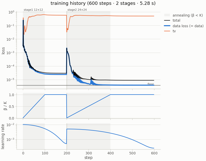
\[ \chi \;=\; \frac{\mathrm{RMSE}\big(F(\hat x),\, y\big)}{\sigma}: \qquad \chi \approx 1 \text{ — explained to the noise}, \quad \chi \gg 1 \text{ — not converged or mis-modelled}, \quad \chi < 1 \text{ — fitting noise}. \]

Training history of the EIT instance: total, data and TV losses on a log scale with the noise floor, the annealing progress and the learning rate over two stages — Training dynamics of `eit` (gallery run): the data loss descends to the noise floor in the second stage; shaded bands mark annealing, the lower panels the annealing progress and the cosine learning-rate schedule.

Instances: complete, reproducible problems¶

An instance packages a full problem behind one protocol: a config dataclass (every paper number is a field), a domain, a scene generator with difficulty classes, an independent data generator, the problem builder, a default curriculum, metrics and baselines. The command line, the benchmark harness, the auto-tuner, the diagnostics and the gallery all drive instances through that protocol, so a new instance gets all of them for free. There are 17 registered instances; tutorial 4 writes a new one.

Vocabulary¶

Inverse crime: Simulating the benchmark data with the very operator used for the inversion. Errors of the discretization cancel, and results look better than they will on real data. Every nefi instance generates data with an independent model — a finer grid, float64, a different scheme (for example an explicit substepped heat simulator against the implicit inversion solver).
Fidelity tag: A string on every operator and data generator ("blur-2x-float64" vs "blur-1x-float32"). The benchmark refuses to run when the two are equal, unless the matched-operator regime is requested explicitly — and then every report labels it.
Cross-fidelity: The default benchmark regime: data from the high-fidelity generator, inversion with the working operator. It exposes the model-error floor: even the ground truth does not fit the data exactly.
Filtering view: A gradient step on the parameters realizes the image-space update \(\Delta x \approx -\eta\, G_\theta \nabla_x \mathcal L\) with \(G_\theta = J_\theta J_\theta^\top\) (NeTMY Lemma 2). The representation filters every update; a free grid (\(G_\theta = I\)) executes the raw gradient, center bias and all. See The representation is the prior.
Gauge: A direction of the unknown that the data cannot see — an additive constant under a mean-free fidelity, a global scale under a normalized one, a global phase in holography. The auto-tuner detects gauges and fixes them in the model.
Data-fit paradox: A reconstruction can fit the data better than the ground truth by absorbing model error into spurious structure (NeFTY App. G.2). A good data fit certifies consistency with the measurement, not accuracy; the diagnostics report it.
Homogeneity: An operator is homogeneous of degree \(p\) if \(F(c\,x) = c^p F(x)\). It enables the energy-anchored scale correction of normalized fidelities (NeTMY Eq. 30) and the automatic data-matched initialization of from_forward.
Smoke preset: The small configuration of an instance (nefi run <name> --smoke, configs/<name>_smoke.yaml) that finishes in seconds on a CPU. Numbers in the gallery come from smoke presets at reduced budgets; the *_full.yaml / *_paper.yaml configs are sized for a GPU.