poisson_source — source recovery for the Poisson equation (elliptic PDE)

At a glance
Problem	The source of the Poisson equation from sparse, boundary or full observations of the potential
Unknown	source f ≥ 0 (softplus head), 64²
Physics	−κΔu = f with Dirichlet boundaries, solved exactly by a spectral (DST) solver — a hard constraint, never a residual
Measurement	potential u on a random 10 % of the pixels (default), a boundary strip or everywhere; data by finite differences on a 2× grid in float64
Difficulty classes	blobs, points, smooth
Baselines	grid, deep_decoder
Metrics	PSNR · MSE · relative error
Run	nefi run poisson_source --smoke · full: nefi run configs/poisson_source_full.yaml

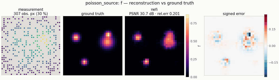
Gallery run (smoke preset: 32², 30 % of the potential observed; 600 steps, 0.6 s on a CPU): PSNR 30.7 dB, all three sources found.

Recover a non-negative source f on the unit square from noisy observations of the potential u

-κ Δu = f  in Ω = [0, extent]²,     u = 0 on ∂Ω,

observed on a sparse random subset of pixels (obs_fraction, default 10 %), on a boundary strip (boundary_width cells) or everywhere. The PDE is a hard constraint: the unknown is f and u is always the exact discrete solution (NeFTY §4.2 design principle), never a soft residual.

from nefi.instances.poisson_source import PoissonSource
inst = PoissonSource(n=64, scene="points", obs_mode="boundary")
out = inst.run(seed=0)
out.metrics                   # {"psnr", "mse", "relative_error"}

CLI: nefi run poisson_source --smoke, nefi run configs/poisson_source_full.yaml. Example: python examples/poisson_source.py [--set obs_mode=boundary --set scene=smooth].

Differentiable spectral solver (nefi.instances.poisson_source.operator)

On the cell-centered grid x_i = (i + ½) h with Dirichlet conditions on the cell faces, the Laplacian's eigenfunctions sin(mπx/L) sampled at the cell centers form the DST-II basis, so

u = IDST-II( DST-II(f) / λ ),   λ_{m,l} = κ [(mπ/Lx)² + (lπ/Ly)²]      (spectrum="continuous")

dst2/idst2 (and the node-centered dst1/idst1) are implemented with real FFTs of odd extensions (torch.fft.rfft/irfft; no scipy in the differentiable path, device-agnostic, batched, any axis; they match scipy.fft.dst(type=2|1) / 2 to 1e-15). PoissonOperator returns the full u grid, is linear (homogeneity = 1), works in 1-3 D and caches eigenvalues per resolution; laplacian(u) applies the inverse map. spectrum="fd" uses the eigenvalues (4/h²) sin²(mπh/2L) of the 5-point Laplacian with antisymmetric ghost cells and therefore reproduces the finite-difference solution exactly.

Observations, masks and coarse stages

The operator predicts u everywhere; the Measurement.mask selects the observed pixels, so the data term is a masked mean (unobserved pixels carry data = 0 and are ignored). Coarse curriculum stages use masked_downsample (installed as InverseProblem.downsample_obs): the coarse datum is the mean of the observed fine pixels in a cell and the coarse mask is the observed fraction (a weight), instead of thresholding an area-averaged binary mask — which would discard most cells of a 10 % random mask.

Data generation (inverse-crime guard) and scenes

PoissonDataGenerator solves the PDE with an independent discretization: a sparse 5-point finite-difference system on a 2× finer grid in float64 (fd_poisson_solve, scipy SuperLU), area- averages u to the native grid, draws the mask with the scene's numpy generator and adds relative Gaussian noise (fidelity_tag = "poisson-fd-2x-float64"; the inversion operator is tagged "poisson-dst-continuous-1x"). Scenes (SourceScenes, cell-averaged, maximum ≈ 1, interior [0.2, 0.8]²): blobs (2-4 compact Gaussians), points (3-6 near-point sources of width point_cells native cells), smooth (broad overlapping blobs).

Prior, objective and curriculum

Neural field with a Softplus (non-negative) or Identity head; data = masked relative MSE (‖pred − obs‖² / ‖obs‖² over observed pixels — scale-free, because u is orders of magnitude smaller than f; data_loss="mse" for the plain masked MSE), l1 and isotropic tv on f. Source recovery is the most ill-conditioned of the three imaging instances ((−Δ)⁻¹ damps frequency k by 1/k²), so first-order methods converge slowly: the default curriculum is 1000 + 2000 steps (with full, low-noise data 450 steps give PSNR 23.3 dB / relative error 0.47, 2000 steps 32.0 dB / 0.17 at 32²).

Configuration (PoissonSourceConfig)

field	default	meaning
n, extent, conductivity	64, 1.0, 1.0	grid, side length, κ
spectrum	continuous	eigenvalues of the inversion solver: continuous | fd
scene, point_cells	blobs, 0.8	blobs | points | smooth; point-source width
obs_mode, obs_fraction, boundary_width	random, 0.1, 3	random | boundary | full
noise_std	0.01	relative to max |u|
supersample	2	FD data-generation grid factor
head, init_value	softplus, 0.05	softplus | identity
data_loss	relative_mse	relative_mse | mse
l1, tv, tv_eps	1e-3, 1e-4, 1e-3	regularizers
hidden, depth, skip_at, n_octaves, activation	128, 4, 2, 6, tanh	neural field
steps, lr, lr_decay, anneal_fraction	(1000, 2000), 1e-2, 0.5, 1.0	curriculum
grid_lr	5e-2	grid baseline
dd_lr, dd_width, dd_stages	5e-3, 64, 5	Deep Decoder baseline

Configs: configs/poisson_source_smoke.yaml (32², 30 % random observations, 200 + 400 steps, ~1-2 s CPU; also the gallery preset), configs/poisson_source_full.yaml (64², 10 %, 2000 + 4000 steps).

The smoke preset changes the prior, not only the size: a ReLU field (activation: relu) with a faster annealing ramp (anneal_fraction: 0.5) and a stronger TV (tv: 5e-4). With the full config's tanh field and anneal_fraction = 1 the compact blobs only become representable at the very end of each stage and the weakest one is never found in a few hundred steps — the optimizer, not the objective, is the bottleneck (the free TV grid with the identical objective recovers it). Over seeds 0-3 the smoke preset gives 30.7 / 29.0 / 28.4 / 28.2 dB (relative error 0.20-0.28) with every blob recovered.

Baselines (PoissonSource.baselines())

grid (free source pixels, same objective) and deep_decoder; any other kind via nefi.baselines.baseline_problem (all keep the mask-aware downsample_obs).

Validation

tests/test_poisson_source.py (≈ 12 s). Measured values:

check	result
DST-I / DST-II vs scipy.fft.dst / 2, round trips, any axis	≤ 1e-12
analytic eigenfunction f = 2π² sin(πx) sin(πy) → u = sin(πx) sin(πy) (n = 32/64/128)	relative error 3.8e-16 / 2.6e-16 / 2.5e-16 (also for extent 2, κ = 0.5)
spectrum="fd" vs scipy sparse 5-point FD	1.4e-14 relative
continuous spectrum vs FD, n = 16 / 32 / 64	1.3e-2 / 3.5e-3 / 8.8e-4 (second order)
torch.autograd.gradcheck through the solver	passes
masked MSE: values at unobserved pixels (data or prediction)	no effect on the loss

Inversion (seed 0, blobs, 1 % noise; baselines at the same step budget):

setting	neural field	grid	Deep Decoder
32², 10 % observed, tanh, 450 steps	22.23 dB / rel. err 0.531 (3.9 s) — 2 of 3 blobs	23.27 / 0.471 (1.3 s)	21.63 / 0.569
32², smoke (30 % observed, ReLU, 600 steps)	30.65 / 0.201 (≈ 1 s) — all 3 blobs	27.96 / 0.274	25.01 / 0.385
64², 1000 + 2000 steps (10 %)	27.57 / 0.315 (185 s*)	29.96 / 0.239 (20 s*)	32.08 / 0.187 (233 s*)

(* wall-clock on a CPU, indicative only.) Source recovery through the smoothing (−Δ)⁻¹ rewards strongly smoothing parameterizations: at the full config the Deep Decoder's global low-pass G_θ fits the compact blobs best and the TV grid beats the tanh neural field; with no explicit prior the grid is still regularized by early stopping (docs/baselines.md). The smoke preset's ReLU field with a short annealing ramp reverses the ranking at 32². Single seed per row — use nefi bench for CIs and the points / boundary regimes.

Notes and limitations

• Homogeneous Dirichlet conditions on a rectangle only (the DST diagonalizes exactly that); other boundary conditions need DCT variants or an iterative solver (nefi/operators/pde).
• Constant conductivity; a spatially varying κ(x) turns this into the Darcy/EIT-type coefficient problem.
• With boundary-strip observations the problem is severely ill-posed (only the far field of the sources is seen); expect depth/size ambiguity rather than sharp recovery.