diffraction_tomography — Born / Rytov inversion of a weak scattering contrast

At a glance
Problem	The scattering contrast of a weakly scattering object from fields measured on a ring of receivers
Unknown	contrast χ = n²/nb² − 1 (bounded head), 32²
Physics	first-order Born (or Rytov) scattering with the 2-D Helmholtz Green's function
Measurement	complex scattered fields for 16 plane-wave illuminations × 64 receivers; data by iterated Lippmann–Schwinger (multiple scattering) on a 2× grid in float64
Difficulty classes	blobs, cells
Baselines	backpropagation (filtered backpropagation), grid
Metrics	PSNR · SSIM · relative error
Run	nefi run diffraction_tomography --smoke · full: nefi run configs/diffraction_tomography_full.yaml

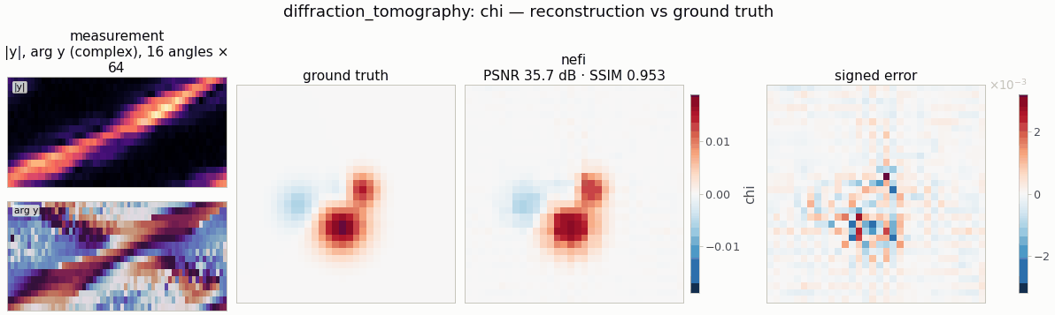
Gallery run (32², 500 steps, 0.7 s on a CPU): PSNR 35.7 dB.

Recover the contrast χ(x) = n(x)²/n_b² − 1 of a weakly scattering object on a square domain (side extent μm, centered) from the complex scattered fields measured on a ring of receivers for n_angles plane-wave illuminations (time dependence e^{−iωt}, k0 = 2π n_b/λ):

Born:   u_s(x_r; θ) = k0² Σ_j G(x_r − y_j) χ_j e^{i k0 d̂_θ·y_j} ΔA,    G = (i/4) H0⁽¹⁾(k0 r)
data:   (2, n_angles, n_receivers) = (Re u_s, Im u_s) + noise

from nefi.instances.diffraction_tomography import DiffractionTomography
inst = DiffractionTomography(scene="cells", n_angles=8, rytov=True)
out = inst.run(seed=0)
out.metrics                                   # {"psnr", "ssim", "relative_error"}
fbp = inst.backpropagation(out.measurement)   # closed-form filtered backpropagation

CLI: nefi run diffraction_tomography --smoke, nefi bench configs/diffraction_tomography_full.yaml --methods neural,backpropagation,grid. Example: python examples/diffraction_tomography.py.

Physics and discretization

• Operator — nefi.physics.scattering.BornOperator (linear, homogeneity = 1): receivers by quadrature with a precomputed Hankel matrix (receivers lie outside the domain → no singularity); rytov=True returns the first-order Rytov phase u_s/u_inc. Rebuilt per curriculum resolution.
• Data generation (inverse-crime guard) — LippmannSchwingerOperator on a 2× finer grid in float64: the total field solves u = u_inc + G ∗ (k0² χ u) by fixed-point (Born-series) iteration with FFT convolution against the Vico–Greengard–Ferrando truncated Green's function (point-source accuracy 0.16 % at λ/8); the scattered field of the total field is then measured. At the default contrast (χ_max = 0.02 over 4λ) the Born model differs from the data by ≈ 3 %. Tags: generator lippmann-schwinger-iterated-2x-float64, inversion born-1x (rytov-1x).
• Scenes (DiffractionTomographyScenes, analytic): blobs (2-4 Gaussian inclusions, mostly positive, one in four negative at half amplitude), cells (2-3 elliptical cells with smooth edges at 0.5·contrast and nuclei at contrast).

Prior, objective and curriculum

Neural field with a Bounded(chi_min, chi_max) head started at χ = 0 (the homogeneous background); fit = relative MSE on the stacked real/imaginary data, tv = isotropic TV. Two-stage multiscale curriculum n/2 → n (NeTMY schedule). The Born operator is linear, so the neural field's role is purely the prior: the implicit smoothing of the MLP plus TV against noise and the missing spatial frequencies (only |K| ≤ 2k0 is measured — the Ewald disk).

Configuration (DiffractionTomographyConfig, defaults = smoke preset)

field	default	meaning
n, extent, wavelength, background_index	32, 4.0 μm, 1.0 μm, 1.0	grid and optics
scene, contrast	blobs, 0.02	phantom class, peak χ
n_angles, n_receivers, receiver_radius	16, 64, 3.0 μm	illuminations, ring receivers
rytov	false	Rytov data model
noise_std, supersample	0.01, 2	noise (× max
ls_iterations, ls_tol, ls_relax	200, 1e-10, 1.0	Lippmann–Schwinger solver
chi_min, chi_max	−0.05, 0.1	head range
hidden, depth, n_octaves	64, 4, 5	neural field
tv, steps, lr, lr_decay, grid_lr_mult	1e-3, (200, 300), 2e-2, 0.5, 1	objective / optimization

PRESETS["full"] / configs/diffraction_tomography_full.yaml: 96² over 8 μm, 64 illuminations × 192 receivers, 256 × 6 MLP, 1500 + 3500 steps.

Smoke results (CPU, seed 0)

scene	zero field	filtered backprop.	grid	neural field
blobs (PSNR / SSIM)	18.6 / 0.54	37.4 / 0.92	36.1 / 0.89	35.7 / 0.95
cells	13.8 / 0.50	26.3 / 0.66	27.5 / 0.79	27.7 / 0.87

(≈ 1 s per neural-field run on a CPU.)

With full-view, densely sampled data and smooth phantoms, filtered backpropagation is a strong classical baseline (the data determine the Ewald disk almost completely); the neural field matches it on smooth blobs and wins on piecewise-smooth cells (TV + MLP prior). Its advantage grows with sparser angles (n_angles: 4-8), limited view, or higher noise, where FBP streaks.

Baselines

grid (free pixels, same objective), backpropagation (Devaney's filtered backpropagation for the circular full-view geometry, wrapped as a closed-form "direct" problem: problem.meta = {"solver": "direct", "reconstruct": fn} for nefi.baselines.solve).