Thermal tomography — NeFTY¶
| At a glance | |
|---|---|
| Problem | Volumetric thermal diffusivity of a slab from its front-surface temperature after a laser flash (pulsed-thermography NDE) — NeFTY, arXiv 2603.11045 |
| Unknown | α(x, y, z) ∈ [αmin, αmax] (bounded sigmoid, NeFTY Eq. 6); 64 × 64 × 16 at paper scale |
| Physics | implicit-Euler finite-volume heat equation with harmonic-mean faces; discrete-adjoint gradients (heat solver) |
| Measurement | 100 surface frames × 64², simulated by an independent explicit substepped solver (float64) |
| Difficulty classes | homogeneous, layered bulk with 1–4 defects (ellipsoids, cylinders, boxes) |
| Baselines | grid (Grid Opt.), pinn_soft (soft-constrained PINN), ppt, tsr (thermography heuristics) |
| Metrics | IoU · Edge F1 · PSNR · SSIM · MSE, plus 2-D IoU / Dice and 2.5-D depth metrics |
| Run | nefi run thermal_tomography --smoke · paper scale: nefi run configs/thermal_tomography_paper.yaml --device cuda |
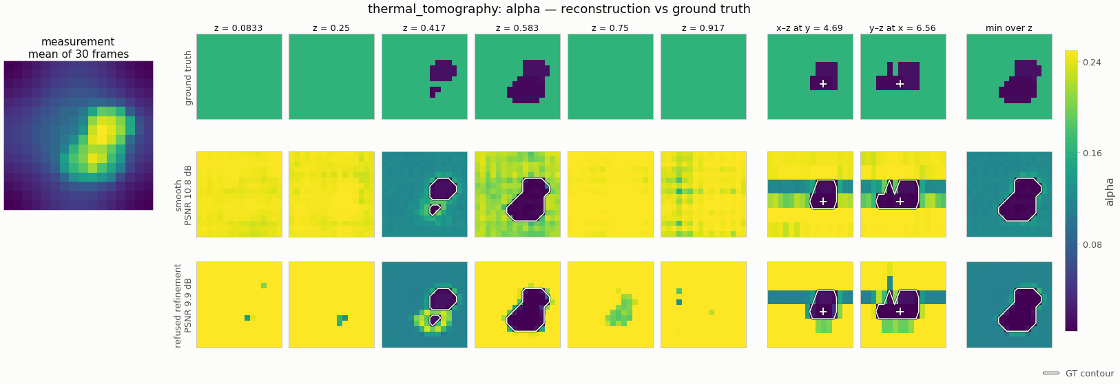
Gallery run (smoke preset 16 × 16 × 6, 30 frames; 600 steps, 6.1 s on a CPU): defect IoU 0.98. The low PSNR (10.8 dB) is a bulk bias from model error; the edge refinement was refused.
nefi.instances.thermal_tomography implements NeFTY (Zhong, Hu, Zheng, Sood, Allen-Blanchette,
Neural Field Thermal Tomography, arXiv 2603.11045): label-free recovery of the volumetric thermal
diffusivity α(x, y, z) of a slab from the transient front-surface temperature after a laser
flash (pulsed-thermography non-destructive evaluation). The PDE is a hard constraint: at every
optimization step the candidate field is pushed through a differentiable implicit-Euler heat solver,
and gradients come from its discrete adjoint at trajectory-sized memory.
ThermalScenes (App. E.1) ─► ExplicitHeatSimulator (forward Euler, N_sub substeps, float64) ─► T̂ (100, 64, 64)
coords ─► annealed Fourier PE (K = 12, no raw x) ─► MLP 10×512 ReLU, skip at 4 ─► α = α_min + (α_max − α_min) σ(f)
      ─► HeatOperator: L(α) harmonic faces, A(α) = I − Δt L(α), 50 Jacobi sweeps/step, adjoint gradients
      ─► surface MSE + λ·TV(α) (Eq. 22) ─► Adam 5e-5, ×0.1 / 1000 steps, 10 000 steps, annealing over 2 500
      ─► metrics (MSE, PSNR, SSIM, IoU@0.03, Edge F1) + surface-fit PSNR + App. H 2-D / 2.5-D projections
Quick start¶
from nefi.instances.thermal_tomography import ThermalTomography

inst = ThermalTomography(preset="smoke")          # 16×16×6, 30 frames, 150 steps (≈ 4 s CPU)
out = inst.run(seed=0, device="cpu")
print(out.metrics)   # mse, psnr, ssim, iou, edge_f1, iou_2d, dice_2d, depth_*, surface_psnr(_init), ...
python examples/thermal_tomography.py --config configs/thermal_tomography_smoke.yaml   # PNGs in runs/
python examples/thermal_tomography.py --config configs/thermal_tomography_smoke.yaml --baseline grid
nefi run thermal_tomography --smoke --plot                                             # via the CLI
python examples/thermal_tomography.py --config configs/thermal_tomography_paper.yaml --device cuda
                                               # paper scale (the paper config compiles the sweeps)
The example writes alpha_slices.png (GT / recovered / |error| per depth slice),
surface_frames.png (observed / re-simulated / residual), projections.png (App. H masks and depth
maps), loss.png, metrics.json, config.yaml and result.pt.
Physics (NeFTY §3.1, App. A)¶
- Diffusivity form (Eq. 1–2):
∂_t T = ∇·(α∇T)withα = k/(ρC_p)onΩ \ Σ; the distributional heat-capacity term on defect interfaces is dropped (App. A.2), so NeFTY solves for a single effective fieldα. - Harmonic-mean faces (Prop. 1): continuity of the effective flux
−α∂_n Tacross a face between constant cells givesᾱ_{i+1/2} = 2α_iα_{i+1}/(α_i + α_{i+1}), dominated by the insulating side (App. A.4).face_mode="arithmetic"is the leaky ablation (Tab. 3 "HM"). - Initial / boundary conditions (App. A.5), with temperatures shifted by the ambient (App. D.2):
- synthetic: Gaussian post-flash
T0 = A exp(−r_xy²/2w_xy²) exp(−z²/2w_z²), periodic lateral faces, adiabatic front and back faces; - real PVC: near-uniform flash
T0 = A exp(−z²/2w_z²), convective Robin back facen·(α∇T) = −hT, lateral periodic or adiabatic.
Initial conditions are stored as exact cell averages (erf integrals), so the deposited heat is
identical at every resolution (a point-sampled w_z = 0.1 flash loses ~9 % of its heat at 4 z-cells
and ~80 % at 2), which keeps coarse multiscale stages and supersampled data consistent. A, w_xy,
w_z are not reported in the paper (defaults 100, 2.5, 0.2; a surface range of ≈ 90 is consistent
with the Tab. 7 surface PSNRs; w_z = 0.2 rather than 0.1 because the thinner layer roughly
triples the model error of implicit Euler relative to the defect signal, see "Inverse-crime
guard").
* Ill-posedness (Prop. 2, Cor. 1): singular values of the linearized map decay algebraically, so
the neural-field prior, frequency annealing and TV are all load-bearing.
Discretization (NeFTY §4.2, App. D.2) — nefi/operators/pde/stencil.py¶
- Grid convention: the unknown lives on the trailing
ndimaxes, the last axis is depthz, and the observed surface is the first sliceT[..., 0]. 2-D(x, z)and 3-D(x, y, z)slabs are supported; leading dims ofTare batch dims. - Operator (Eq. 7):
[L(α)T]_i = Σ_d Δ_d⁻² (ᾱ_{i+1/2}(T_{i+1} − T_i) − ᾱ_{i−1/2}(T_i − T_{i−1})) − β_i T_i. Implemented withtorch.rollon precomputed face conductancesa = ᾱ/Δ²(computed once per forward fromα, reused by allN_t × Kinner iterations); fully autodiff-compatible and device-agnostic. - Boundary conditions (
BoundarySpec, one kind per axis):"periodic"— circular wrap;"neumann"— zero conductance on the boundary face, exactly equivalent to the replicate padding of App. D.2 (zero cross-face increment);"robin"(last axis only) — adiabatic front face and back-face sinkβ = h/Δzfrom the finite-volume flux balance (App. D.2). - Implicit Euler (Eq. 8):
A(α)T^{n+1} = T^n,A = I − ΔtL(α).Ais symmetric, has unit row-sum excessA_pp − Σ|A_pq| = 1 + Δtβ_p ≥ 1(strict diagonal dominance) and is SPD withλ_min(A) ≥ 1— all checked numerically on dense matrices in the tests for periodic, adiabatic and Robin boundaries. - Inner solvers (
linear_solvers.py):jacobi(apply_A, diag, b, x0, iters)— Eq. (24), warm-started from the previous frame; the operator uses the algebraically identical fused sweepx ← D⁻¹b + Σ_j W_j ⊙ shift_j(x).conjugate_gradient(apply_A, b, x0, tol, max_iter)— Jacobi-preconditioned CG. At the paper spacing andΔtthe Jacobi contraction is ≈ 0.84–0.89 per sweep;K = 50gives a relative error of 3.0e-6 on the sharpest right-hand side (the first post-flash step) and 3.0e-5 accumulated over 100 frames (float64, vs. CG at 1e-13). - Substeps (
implicit_substeps, default 1 = paper):mimplicit steps ofΔt/mper frame.
Discrete adjoint (NeFTY §4.3, App. D.3) — nefi/operators/pde/adjoint.py¶
ImplicitEulerAdjoint is a torch.autograd.Function:
- forward runs the recurrence without autograd and saves only the detached trajectory
T^1..T^{n_last}(O(N_g N_t), viasave_for_backward, sotorch.autograd.graph.save_on_cpucan offload it to host memory); - backward runs
A μ^n = μ^{n+1} + ∂ℓ^n/∂T^n,μ^{N_t+1} = 0(Eq. 10 / 26) backwards in time with the same inner solver (Aᵀ = A), injecting the frame gradients at the surface, and returnsdJ/dα = Δt Σ_n (μ^n)ᵀ ∂(L(α)T^n)/∂α(Eq. 11 / 27) anddJ/dT^0 = μ^1(initial-condition sensitivity, App. D.3). Steps after the last observed frame are skipped (theirμvanishes). - gradient assembly:
μᵀL(α)T = −Σ_faces a_f(α)(Δ_fμ)(Δ_fT) − Σβμ Tis bilinear, so the defaultadjoint_assembly="fused"accumulatesS_f = Σ_n (Δ_fμ^n)(Δ_fT^n)during the sweep and back-propagates through the face conductancesa_f(α)once (this contains the harmonic-mean derivative∂ᾱ/∂α_i = 2α_{i+1}²/(α_i + α_{i+1})²)."per_step"runs one small autograd VJP ofα ↦ L(α)T^nper step — the literal Eq. (27); both agree to 1e-13.
HeatOperator(grad_mode=...) selects "adjoint" (default), "autograd" (back-propagation through
the unrolled inner solver — the reference) or "checkpoint" (torch.utils.checkpoint per time
step). The adjoint differentiates the exactly solved recurrence (App. D.2 treats T^(K) as the
exact state), whereas autograd differentiates the truncated K-sweep map; the two differ by
O(ρ^K) with ρ the Jacobi contraction (≈ 1e-3 relative for K = 10 on the smoke grid, ≤ 1e-6 for
converged solves). Saved-tensor accounting (test test_adjoint_memory_is_trajectory_sized, float32 grids):
| mode | saved tensors | 64×64×16, K = 50: N_t = 50 (Tab. 4 setting) / N_t = 100 |
|---|---|---|
| adjoint | (N_t + 1)·N_g (trajectory + α) |
13.4 MB / 26.5 MB (paper Tab. 4: 21.9 MB) |
| checkpoint | ≈ 9.6·N_t·N_g + one step's recomputation |
0.13 GB / 0.25 GB, + 0.16 GB |
| autograd | ≈ 12·K·N_t·N_g |
7.9 GB / 15.7 GB (paper Tab. 4: 18.6 GB) |
compile_solver=True (HeatOperator(compile=True)) runs the gradient-free Jacobi sweeps of the
adjoint forward/backward through torch.compile (bit-identical; 3.2× faster per solve on a
CPU after a ~30 s one-time compile; compile_mode="reduce-overhead" adds CUDA graphs, with
the solve output cloned out of the graph pool — untested on CUDA). It is on in
configs/thermal_tomography_paper.yaml (one-time compile of tens of seconds) and off in the code
default, so CPU / MPS / tests stay eager.
Eager sweeps use a flat padded layout (stencil_backend="auto", see
performance): one gather refills the periodic ghost cells and six addcmul
run on contiguous views — 7 kernels per sweep instead of 12 with torch.roll, same numbers to
float rounding, 2.3× faster smoke steps on CPU, 4.5× less memory in grad_mode="autograd".
solver="chebyshev" (opt-in) accelerates the same sweeps with the Chebyshev semi-iteration
(Gershgorin bound, no host sync): ≈ 20 iterations match the error of the paper's 50 Jacobi sweeps
at the Tab. 5 time step (12–13 vs 20 on the smoke grid).
Inverse-crime guard (NeFTY §5.1, App. E.1)¶
Data are generated by ExplicitHeatSimulator (fidelity_tag="explicit-substepped-float64"), which
shares no time-stepping or boundary code with the inversion operator: ghost cells by circular /
replicate padding, flux-difference divergence, forward Euler with
N_sub = max(10, ⌈Δt/Δt_stable × 2⌉), Δt_stable = Δx_min²/(2Dα_max) substeps per frame
(16 / 24 / 31 at the paper grid for α_max = 0.1 / 0.15 / 0.2), float64. Optional
sim_supersample simulates on a finer grid and area-averages.
Model mismatch is real and large at the paper's settings. Implicit Euler at one step per camera
frame under-resolves the fast through-thickness decay of the thin post-flash layer: for the paper
grid with w_z = 0.1 the surface mismatch against the substepped explicit data is ≈ 10 % (relative
rms) in frame 1, 2.8 % in frame 10 and 0.3 % in frame 90, i.e. ≈ 40 % of the rms defect signal of a
two-defect test scene (w_z = 0.2, the default: 14 %; w_z = 0.1 skipping the first 5 frames: 13 %).
For the paper preset (seeds 0–2) the model-error floor — the surface MSE of the ground truth
re-simulated by the inversion operator — is 0.18–0.21 at w_z = 0.1 and 0.07–0.09 at w_z = 0.2,
against an initial uniform-field MSE of 0.46–13.6 (mostly set by the bulk value): at w_z = 0.1 the
defect signal of some scenes barely exceeds the model error. Check this ratio first when paper-scale
results are poor. The inversion compensates by inflating α near the front face (visible in
alpha_slices.png) and slightly in the bulk (smoke preset:
+0.02 median bias at Δt = 0.1, +0.04 at Δt = 0.2). Knobs: implicit_substeps (error O(Δt/m)),
first_frame (drop the earliest frames), flash_width_z. Because even the ground truth
re-simulated by the inversion operator stays at the model-error floor (≈ 46 dB surface PSNR at
w_z = 0.1, ≈ 50 dB at w_z = 0.2, surface range ≈ 90), the ≈ 82 dB of Tab. 7 is not reproducible
under this inverse-crime guard; the smoke runs reach 37–45 dB.
Instance (nefi/instances/thermal_tomography/)¶
ThermalTomography(cfg=None, preset=None, **overrides)— registered as"thermal_tomography"; presets"paper"(defaults),"layered","smoke"(PRESETS).field()—NeuralField(3, {"alpha": Bounded(α_min, α_max, init_value=α_init)}, hidden=512, depth=10, skip_at=4, activation="relu", n_octaves=12, include_input=False)(2.44 M parameters, as in Tab. 9).losses()—{"data": MSE(), "tv": TV("alpha", isotropic=True, eps=1e-6, periodic_axes=(0, 1))}, weights{data: 1, tv: 1e-3}. TV follows Eq. (22): lateral periodic forward differences, zeroδzon the last slice, physical spacing, mean reduction. Convention: the paper writes the data term as a sum overM·N_Γsurface samples and TV as a volume integral; with per-element means the equivalent weight would beλ|Ω|/(M N_Γ) ≈ 2.4e-7. nefi keeps the mean/mean form withλ = 1e-3(temperatures in units of the flash amplitudeA = 100), which makes TV active at the converged data-misfit level; tunetv_weightwhen changingflash_amplitude(MSE scales withA²).default_curriculum()— single stage (paper): Adam,lr 5e-5, step decay ×0.1 every 1000 steps, 10 000 steps, annealing over the first 2 500 (anneal_fraction = 0.25), no weight decay, no clipping.n_stages > 1gives a coarse-to-fine curriculum (at_resolutionrebuilds spacing and the initial condition;surface_downsamplearea-averages the frames laterally).baselines()["grid"]— Grid Opt. (App. F.2):GridField+ the same bounded head, solver, adjoint, TV and schedule, initialized at the bulk guess (grid_lr,grid_stepsoverride).baselines()["pinn_soft"]— soft-constrained PINN (Eq. 4, App. F.1,pinn.py): a tanh temperature surrogateT_φ(x, t)is the problem's operator (SoftPINNSurface, its parameters are optimized with the field), the α network is NeFTY's field, and the losses are the scale-normalized surface MSE, the PDE residual∂_tT_φ − α_θΔT_φ − ∇α_θ·∇T_φatpinn_collocationrandom space-time points (autograd derivatives) and the initial-condition misfit. Weights are fixed (pinn_lambda_pde,pinn_lambda_ic) instead of GradNorm. Since the predicted frames do not depend onθ,∇_θ L_data ≡ 0— the §3.3 decoupling, verified in the tests: on the smoke measurement the data loss drops 33× in 150 steps whileα_θstays uniform (std 0.0025, IoU 0, Edge F1 0).make_measurement(seed, scene_class)— draws a scene, simulates it with the explicit simulator, adds optional noise (noise_std, relative; the paper's synthetic data are noise-free) and stores the bulk field, defect mask and scene parameters inmeasurement.meta.evaluate(result, gt, measurement=None)—mse,psnr(rangeα_max − α_min),ssim(slice-wise along z),iou(α < 0.03),edge_f1; App. H projectionsiou_2d,dice_2d,depth_abs_rel,depth_rmse,depth_delta1; with the measurement alsosurface_psnr/surface_mseof the recovered field's re-simulation andsurface_psnr_initof the initial uniform field (data-fit-paradox diagnostic, §5.2 / App. G.2).
Scenes (ThermalScenes, App. E.1): classes homogeneous (bulk U(0.1, 0.2)) and layered
(3–4 strata along z, independent bulk values); 1–4 ellipsoid / cylinder (circular, axis along z) / box
defects with α ~ U(0.005, 0.015) at random depths, laterally wrapped on periodic slabs. Parameters are
drawn first and rasterized analytically at any shape. Defect sizes/depths are not given in the
paper (defect_radius_range, defect_half_thickness_range, defect_depth_range).
Projections (projection.py, App. H.3): defect_mask_2d (depth-averaged deficit
[1 − ᾱ/α_base]_+ > 2σ̂) and depth_map_25d (median depth of the flagged voxels of each masked
pixel). α_base may be a scalar, a depth profile or None (label-free estimate: lateral median per
depth slice). Deviation: the noise floor σ̂ = 1.4826·MAD is computed from the signed deficit;
the MAD of the clipped deficit (the literal text, mad_of="clipped") collapses to ~0 whenever more
than half of the pixels are sound, flagging about half of them (shown in the tests).
Metrics (nefi/metrics/segmentation.py): iou_below, edge_f1 (gradient magnitude thresholded
at 50 % of the GT maximum, precision/recall within a dilate-voxel tolerance band), abs_rel,
depth_rmse, delta_threshold (Eigen et al.), radial_power_spectrum, field_gradient_magnitude,
binary_dilation.
Paper → config → code¶
| Paper item | Value | Config field | Code |
|---|---|---|---|
Domain L × L × H (Tab. 5) |
10 × 10 × 1 | extent |
ThermalTomography.domain |
Grid N_x × N_y × N_z (Tab. 5) |
64 × 64 × 16 (Δx = 0.156, Δz = 0.0625) | grid |
Domain.spacing |
Time step Δt, frames N_t (Tab. 5) |
0.05, 100 | dt, n_frames (first_frame, frame_stride) |
HeatOperator(dt, n_steps, obs_frames) |
| Implicit Euler (Eq. 8) | 1 step / frame | implicit_substeps |
adjoint.rollout |
Jacobi iterations K (Eq. 24, Tab. 5) |
50 | jacobi_iters (solver = jacobi / chebyshev / cg, cg_tol, cg_max_iter, stencil_backend) |
adjoint.solve_step, stencil.ImplicitSystem.jacobi_sweeps |
| Face coefficient (Prop. 1) | harmonic | face_mode |
stencil.face_coefficients |
Bounds (α_min, α_max) (Eq. 6, Tab. 5) |
(0.003, 0.25) | alpha_min, alpha_max |
fields.Bounded |
| Lateral / front-back BCs (App. A.5) | periodic / adiabatic | bc_lateral, bc_back, robin_h |
stencil.BoundarySpec |
| Initial condition (App. A.5) | Gaussian flash | initial, flash_* |
heat.GaussianFlash, heat.UniformFlash |
| Discrete adjoint (Eq. 10–11, 25–27) | — | grad_mode, adjoint_assembly |
adjoint.ImplicitEulerAdjoint |
torch.compile (App. D.2) |
on | compile_solver, compile_mode |
adjoint._compiled_sweeps |
| Bulk / defect α (App. E.1) | U(0.1, 0.2) / U(0.005, 0.015) | alpha_base_range, alpha_defect_range |
scenes.ThermalScenes |
| Defects / strata (App. E.1) | 1–4 / 3–4 | n_defects, n_layers, defect_* |
scenes.ThermalScenes |
| Substeps (App. E.1) | max(10, ⌈Δt/Δt_stable·2⌉) | sim_min_substeps, sim_substep_safety |
heat.explicit_substeps |
| Data engine (§5.1, App. E.1) | independent explicit | sim_face_mode, sim_supersample, noise_std |
heat.ExplicitHeatSimulator |
| MLP depth / width / skip / activation (Tab. 5) | 10 / 512 / 4 / ReLU | depth, hidden, skip_at, activation |
fields.NeuralField |
Encoding bandwidth N (Eq. 20) |
12 | n_octaves, include_input |
fields.FourierFeatures |
| Frequency annealing (Eq. 21) | over 2 500 steps | anneal_steps |
Stage.anneal_fraction |
| Optimizer (Tab. 5) | Adam, 5e-5, ×0.1 / 1000, 10 000 steps | optimizer, lr, lr_schedule, lr_step_size, lr_gamma, steps |
default_curriculum |
| TV weight / smoothing (Eq. 22, Tab. 5) | 1e-3 / 1e-6 | tv_weight, tv_eps |
losses.TV(isotropic=True) |
| IoU threshold (App. E.2) | τ = 0.03 | iou_tau |
metrics.iou_below |
| Edge F1 (App. G.5) | 50 % of GT max | edge_threshold, edge_dilate |
metrics.edge_f1 |
| 2-D mask / 2.5-D depth (App. H.3) | 2σ̂ MAD rule, spatial median | projection_k |
projection.defect_mask_2d, depth_map_25d |
| Grid Opt. (App. F.2) | same schedule | grid_lr, grid_steps |
baselines()["grid"] |
| Soft PINN (Eq. 4, App. F.1) | T_φ 5 × 128, N_c = 24 576, Adam 1e-3, 22 000 it. | pinn_* |
baselines()["pinn_soft"], pinn.py |
| Gaussian variance test (App. I) | slope 2α | — | tests/test_heat_solver.py::test_gaussian_variance_growth |
Validation (tests)¶
tests/test_heat_solver.py (~20 s) and tests/test_thermal_tomography.py (~15 s):
- Gaussian variance growth (App. I, Eq. 30–32): α = 0.1, 64×64×8 periodic/adiabatic slab,
Δt = 0.05, 100 frames, K = 50: surface-moment slope error 0.42 % (< 1 %; the residual is the
first-order time error of the surface slice, 0.09 % at Δt = 0.01); the volume moment grows by exactly
2αΔtper step (rel. error 2.6e-7), and a z-uniform 2-D Gaussian is exact to 1e-6. - Adjoint (6×6×4, 5 frames, float64, CG at 1e-14): adjoint (fused and per-step) and checkpoint
gradients match unrolled autograd to ≈ 3e-13 (periodic, adiabatic, Robin); Jacobi (K = 200) to 2e-15;
torch.autograd.gradcheckpasses for a random quadratic loss w.r.t.αandT0, and for the full Jacobian including the initial frame;dJ/dT0 = μ¹reaches a learnable initial-condition module. - Harmonic vs arithmetic (1:20 insulating layer): the heat rate into the layer is 5.5× smaller and the heat behind it after 30 steps < ½ of the arithmetic case; identical for uniform α.
- Linear solvers: A symmetric (dense check), SPD, diagonally dominant for all BCs; Jacobi (K = 50) vs CG 3e-6 per solve at the paper spacing; CG residual strictly decreasing (with/without preconditioner).
- Boundaries: periodic + adiabatic conserve heat to 1e-11 (CG) / 1e-6 (Jacobi) and wrap
symmetrically; the Robin back face loses heat strictly monotonically;
h = 0recovers conservation. - Multiscale:
at_resolutionkeeps Δt / frames / BCs, rebuilds spacing andT0;output_shapematches;Measurement.resampled/surface_downsampleequal the lateral 2×2 average. - End to end (smoke preset, seed 0, 3.8 s on one CPU core): IoU 0.97 (uniform start: 0), PSNR 16.6 dB,
SSIM 0.54, Edge F1 1.0, surface PSNR 45.1 dB vs 21.6 dB for the initial uniform field. Over seeds
0–4: IoU 0.26–0.97 (mean 0.50), PSNR 15.1 dB; layered scenes (seeds 0–1): IoU 0.46–0.47. The slow
test (seeds 0–1 × 200 steps, ≈ 37 s) reaches IoU 0.98 / 0.25 and asserts a mean ≥ 0.2. Grid Opt.
on the same seed-0 measurement (
--baseline grid): IoU 0, PSNR 14.1 dB, surface PSNR 31.5 dB (paper Tab. 1: IoU 0.04). - Paper network / optimizer proxy (not a test; 10 × 512 ReLU MLP, Adam 5e-5 with ×0.1 / 1000, paper scene and flash on a reduced 32×32×8 grid, 50 frames of 0.1, 600 steps, seed 0): IoU 0.33, PSNR 14.5 dB, Edge F1 0.63, surface PSNR 56.6 dB vs 38.3 dB for the uniform start (lr 5e-4: IoU 0.45); ≈ 1.4 s/step on 2 CPU threads, dominated by the MLP.
Running: CPU vs CUDA server¶
- CPU: use the smoke preset/config (≈ 9 ms per step, 21 ms before the flat stencil).
Tiny stencil ops are overhead bound:
torch.set_num_threads(1)is fastest (the example sets--threads 1). Forward + adjoint at 64×64×16, 20 frames, K = 50 on a CPU: 268 ms (torch.roll, 1 thread) / 454 ms (4 threads) → 197 / 246 ms (flat) → 90 ms (flat + Chebyshev K = 20, 1 thread). Paper scale on CPU remains impractical (≈ 1 s per step for the heat solve single-threaded + several s for the 10 × 512 MLP on 65 536 points). - CUDA server:
configs/thermal_tomography_paper.yamlwith--device cuda(it setscompile_solver: true; the registered instance--set preset=paperneeds--set compile_solver=true). Memory: ≈ 30 MB for the adjoint trajectory plus the MLP activations on 65 536 points (a few GB; the paper reports 4.3 GB peak). Time (estimated, not measured here): each optimization step runs 2 × 100 × 50 = 10⁴ Jacobi sweeps; eager PyTorch launches ~12 kernels per sweep (≈ 0.6–1 s per step, 2–3 h per specimen); withcompile_solver=trueeach sweep fuses into ≈ 1 kernel (≈ 0.1 s per step, ≈ 15–20 min per specimen; the paper reports 57.5 ms/step, 9.6 min).solver="cg"needs fewer matvecs than 50 Jacobi sweeps per solve (2.3× faster forward on CPU) but performs host syncs for its tolerance test (cg_tol=0runs a fixed count without syncs).
Real data: pulsed thermography recordings (NeFTY §5.3, App. H)¶
nefi/instances/thermal_tomography/realdata.py turns a recorded surface sequence into a problem
without touching the simulator:
from nefi.instances.thermal_tomography import ThermalTomography
from nefi.instances.thermal_tomography.realdata import (
    PhysicalScales, load_frames, measurement_from_frames, config_for_frames, pvc_overrides,
    physical_depth_map,
)
from nefi.instances.thermal_tomography.projection import defect_mask_2d, depth_map_25d
import nefi

frames = load_frames("data/pvc/specimen_07.npy")           # (n_t, H, W), any units, local file
meas, meta = measurement_from_frames(frames, dt=1 / 50, pre_flash_frames=5,
                                     resample_to=(64, 64), max_frames=100)
scales = PhysicalScales(alpha_phys=1.2e-7, L0=0.1, thickness=0.005,
                        t_total=meta["t_total_phys"])       # PVC: 100 mm footprint, 5 mm thick
cfg = config_for_frames(meas, scales, nz=16, base=ThermalTomography(preset="paper").config_dict(),
                        **pvc_overrides(scales, robin_h=0.05, lateral="neumann"))
problem = ThermalTomography(cfg).build_problem(meas)
result = nefi.invert(problem, device="cuda")
alpha = result.fields["alpha"]                              # unitless (Fourier number)
mask = defect_mask_2d(alpha, scales.fourier_number)         # App. H.3 MAD rule
depth_mm = physical_depth_map(depth_map_25d(alpha, ...), scales, "mm")
The unitless solver evolves in (t / t_total, x / L0) with α_sim = α_phys · t_total / L0²
(the Fourier number), so the same solver parameters serve micron/microsecond and
centimetre/second specimens; PhysicalScales converts fields, times and depths both ways.
pvc_overrides applies the three App. H.2 adaptations (near-uniform front-face flash, convective
Robin back face, lateral Neumann boundaries on crops) and brackets the diffusivity around the bulk
value. No dataset is bundled — the PVC-Infrared / PVC-Depth benchmarks (Wei et al. 2023) must be
downloaded separately and pointed to by path. The Robin coefficient and the flash amplitude are
calibrated per setup (App. H.2); noise_std="auto" estimates the camera noise for discrepancy
stopping.
Failure modes and limitations¶
- Shallow defects near the flash (App. G.7): surface data are weakly sensitive to the back-face diffusivity, and the optimizer can place a spurious low-α layer along the back face that is consistent with the surface decay. Lateral 2-D masks stay correct, depth metrics suffer. Remedies suggested by the paper: stronger back-face priors, back-face thermograms, depth-adaptive TV.
- Front-face inflation from model mismatch (see "Inverse-crime guard"): expect elevated α in the
first depth slices; use
implicit_substeps/first_frameto reduce it. - High contrast: the 1:20 defect contrast of App. E.1 keeps
Awell conditioned; at air-like contrasts (> 1:1000) Jacobi stalls — switch tosolver="cg"(App. J). - Soft-PINN baseline is minimal: fixed loss weights (no GradNorm), no SPINN / Causal-PINN / DCGD variants (App. C.3 argues they share the same decoupling).