hide: - toc description: The registered physical systems reconstructed by the same recipe: overview figure, per-system comparisons and optimization animations from one gallery run on a CPU.
Gallery
The registered inverse problems, 1-D, 2-D and volumetric, linear and nonlinear, elliptic, hyperbolic, parabolic and spectral, are all solved by the same recipe: a coordinate neural field, the instrument's physics as a hard constraint, a coarse-to-fine curriculum. Every measurement is simulated with an independent, finer model than the one being inverted (no inverse crime), so each reconstruction has to cope with model error as well as noise.
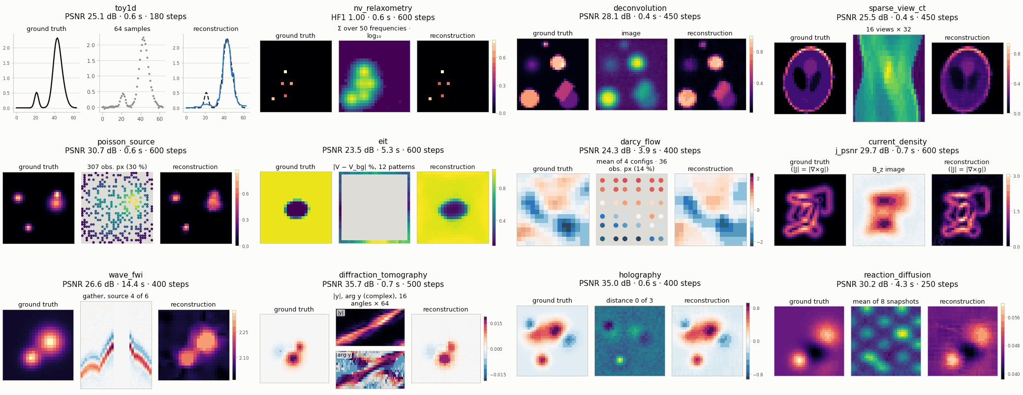
examples/gallery.py (smoke presets at 0.2 × the default
budgets, CPU, 182 s for all systems). The five volumetric systems are on the
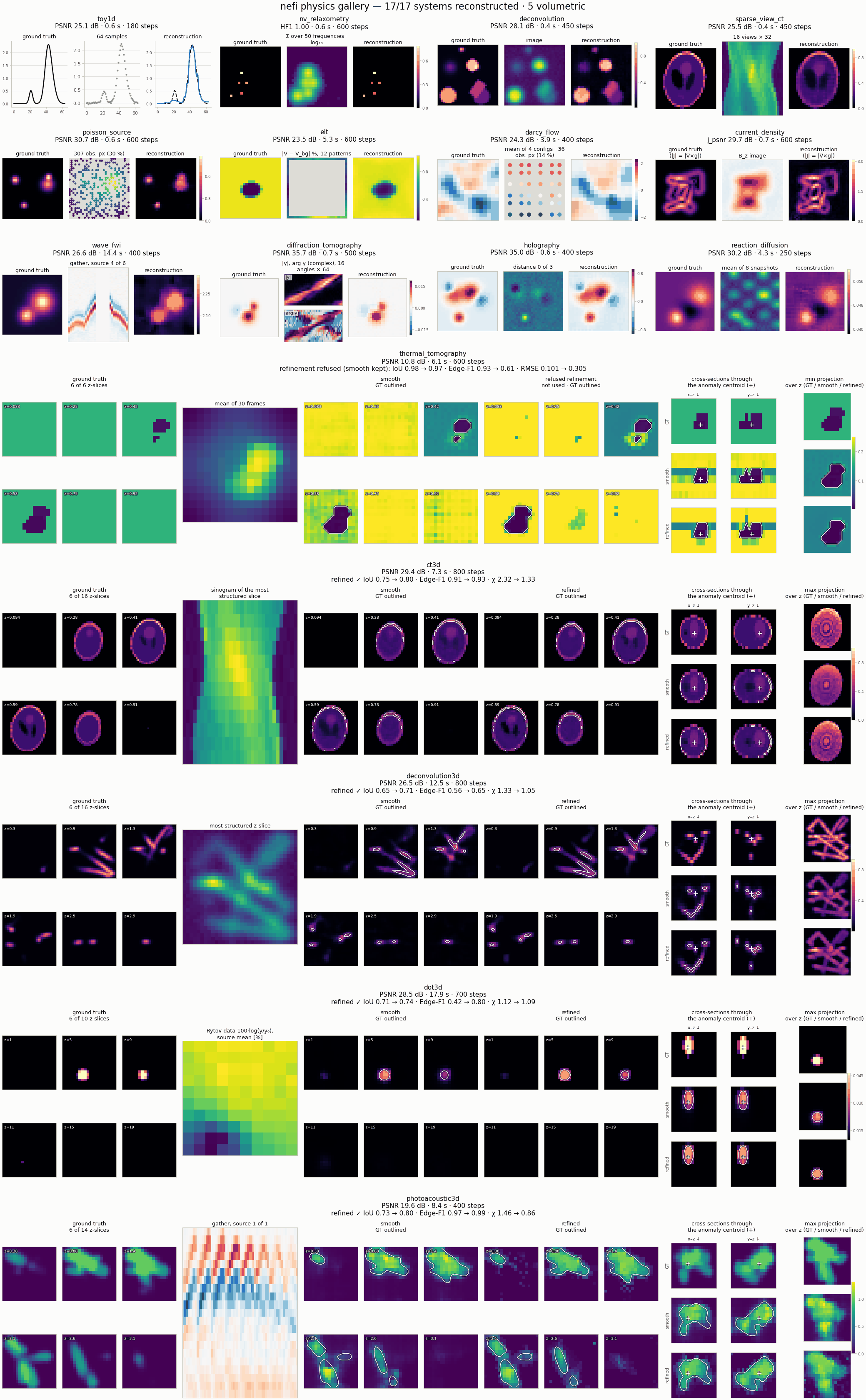
3-D showcase; the full overview of all systems opens at
full resolution. Click any figure to zoom.Legend
Numbers from the run's manifest (runs/gallery/physics/manifest.json): smoke preset, one seed,
0.2 × the default step budget (× 2 for the volumetric systems), CPU with 4 threads, torch
2.11. They show what a few seconds of CPU buy; the instance pages report converged and
paper-scale numbers.
| system | recovered from | grid · steps · solve | result |
|---|---|---|---|
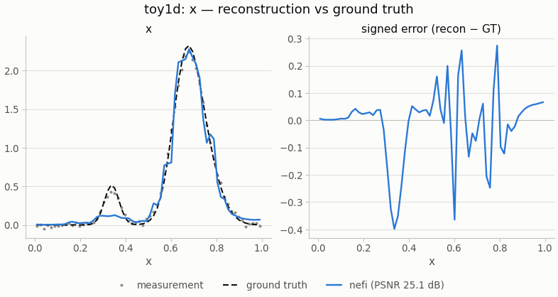
| toy1d | a 1-D signal from 64 blurred samples | 64 · 180 · 0.6 s | PSNR 25.1 dB |
| NV relaxometry · NeTMY | spin sources from noise spectra at 50 frequencies | 24² · 600 · 0.6 s | Hungarian F1 1.00 |
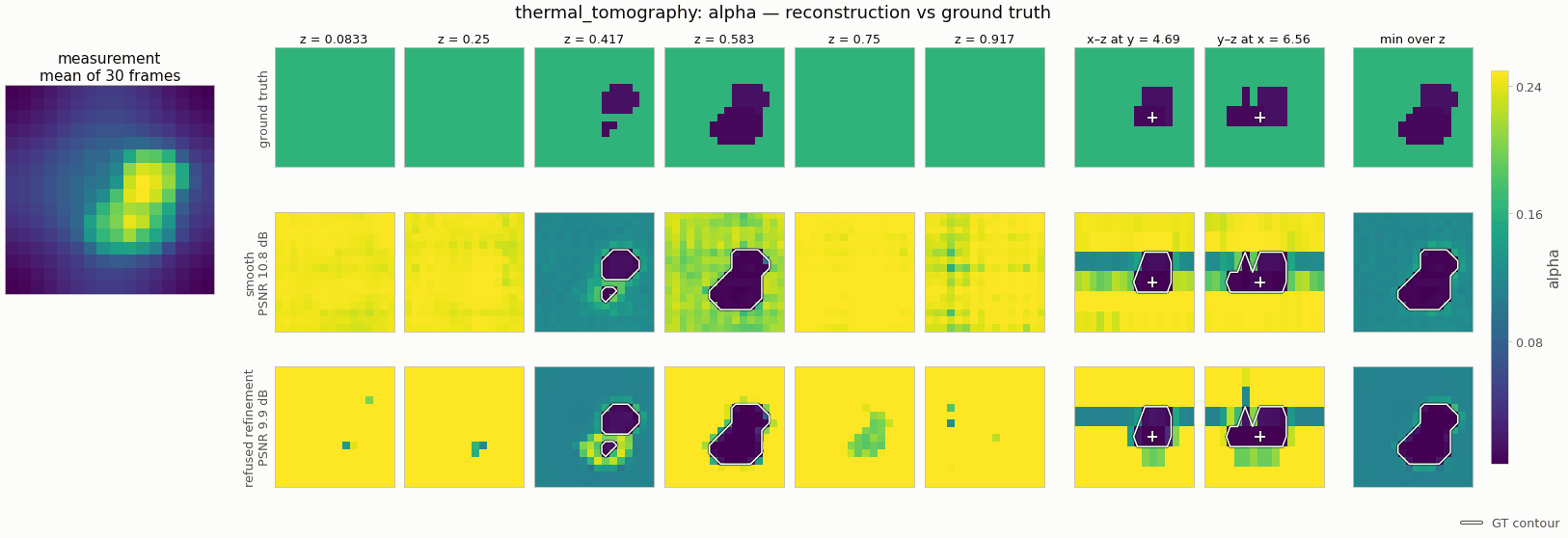
| Thermal tomography · NeFTY | 3-D diffusivity from 30 surface frames | 16²×6 · 600 · 6.1 s | IoU 0.98 · PSNR 10.8 dB |
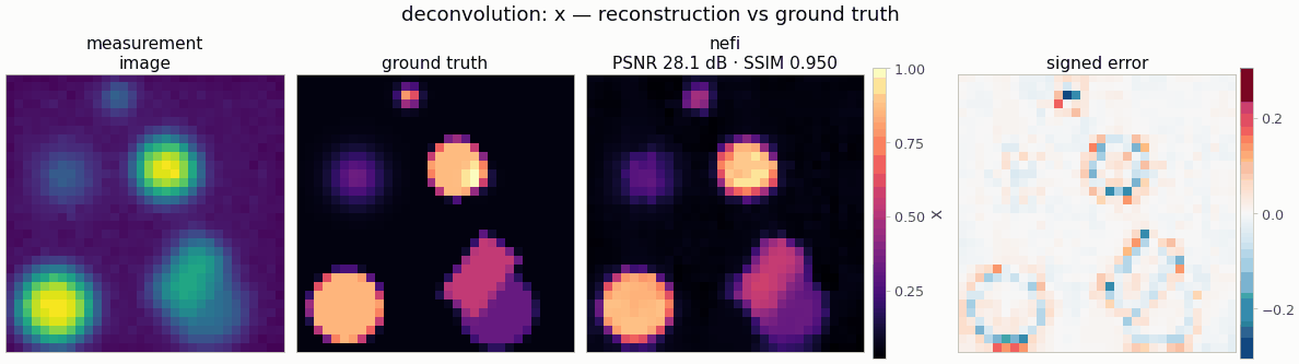
| Deconvolution | an image from its blurred copy | 32² · 450 · 0.4 s | PSNR 28.1 dB |
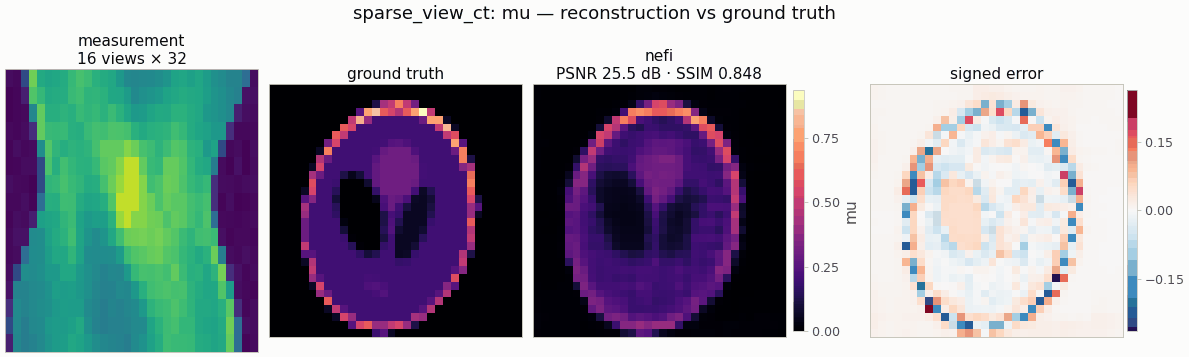
| Sparse-view CT | attenuation from 16 projections | 32² · 450 · 0.4 s | PSNR 25.5 dB |
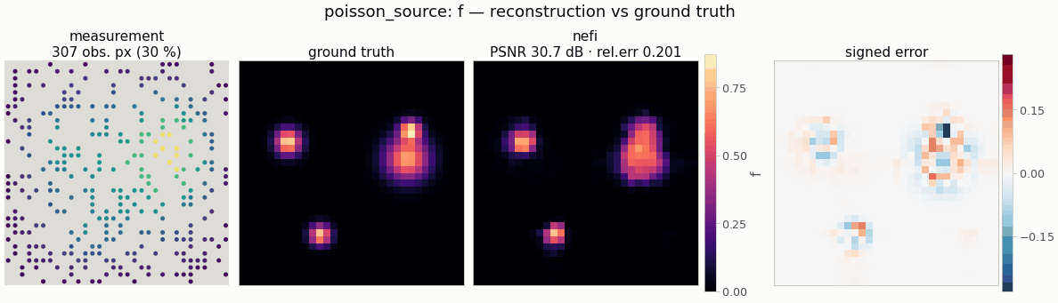
| Poisson source | sources from 30 % of the potential | 32² · 600 · 0.6 s | PSNR 30.7 dB |
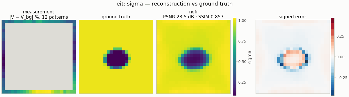
| EIT | conductivity from boundary voltages, 12 patterns | 24² · 600 · 5.3 s | PSNR 23.5 dB · IoU 0.94 |
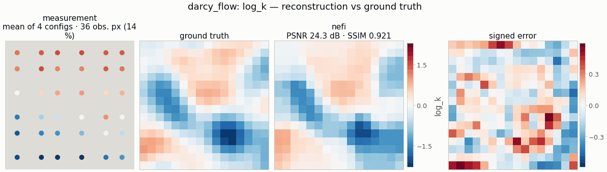
| Darcy flow | log-permeability from well gauges, 4 configurations | 16² · 400 · 3.9 s | PSNR 24.3 dB |
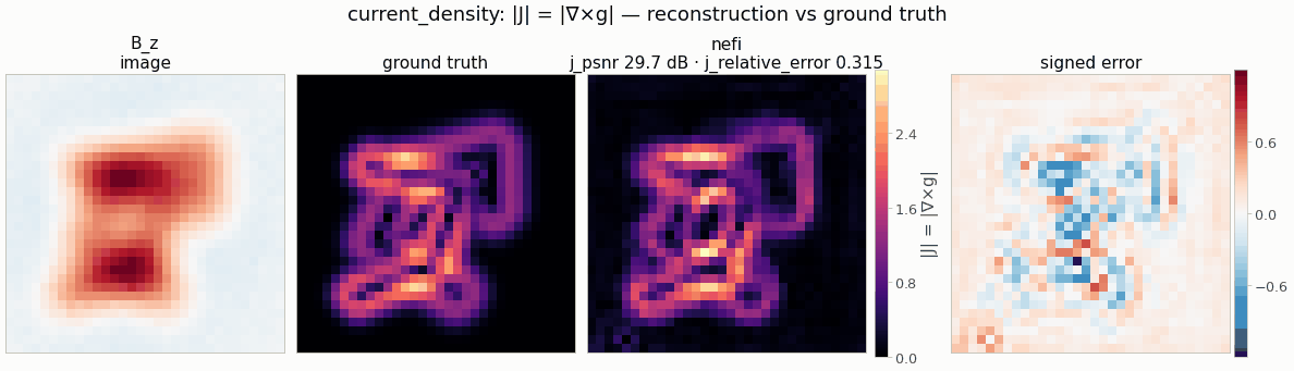
| Current density | a sheet current from its stray field | 32² · 600 · 0.7 s | current PSNR 29.7 dB |
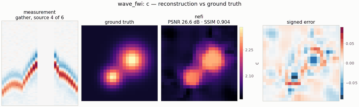
| Full-waveform inversion | sound speed from 6 × 32 acoustic traces | 24² · 400 · 14.4 s | PSNR 26.6 dB |
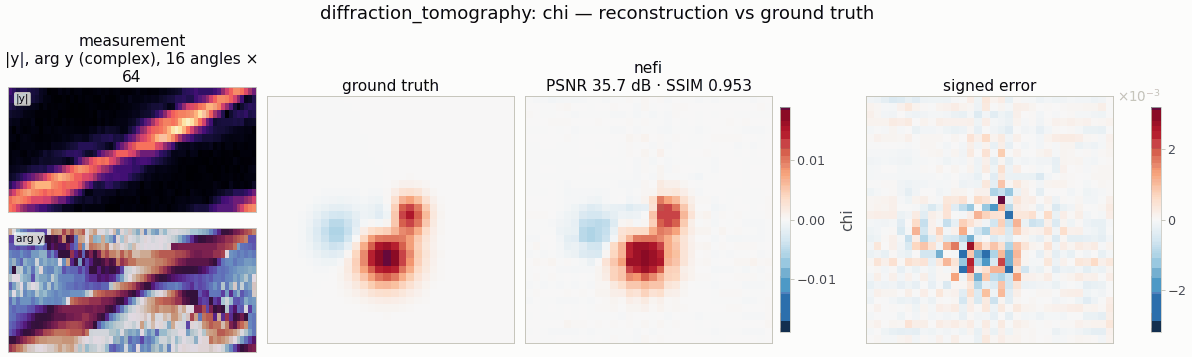
| Diffraction tomography | contrast from complex fields, 16 angles | 32² · 500 · 0.7 s | PSNR 35.7 dB |
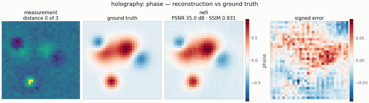
| Holography | phase from intensities at 3 distances | 32² · 400 · 0.6 s | PSNR 35.0 dB |
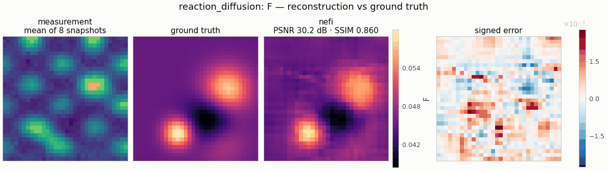
| Reaction–diffusion | the feed rate from 4 snapshots of 2 species | 32² · 250 · 4.3 s | PSNR 30.2 dB |
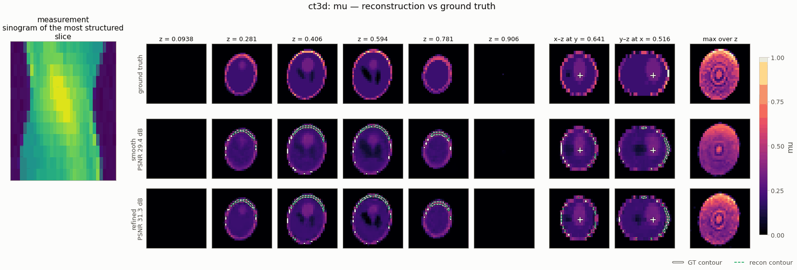
| 3-D CT | attenuation from 12 views of every slice | 32²×16 · 800 · 7.3 s | PSNR 29.4 dB · refined IoU 0.75 → 0.80 |
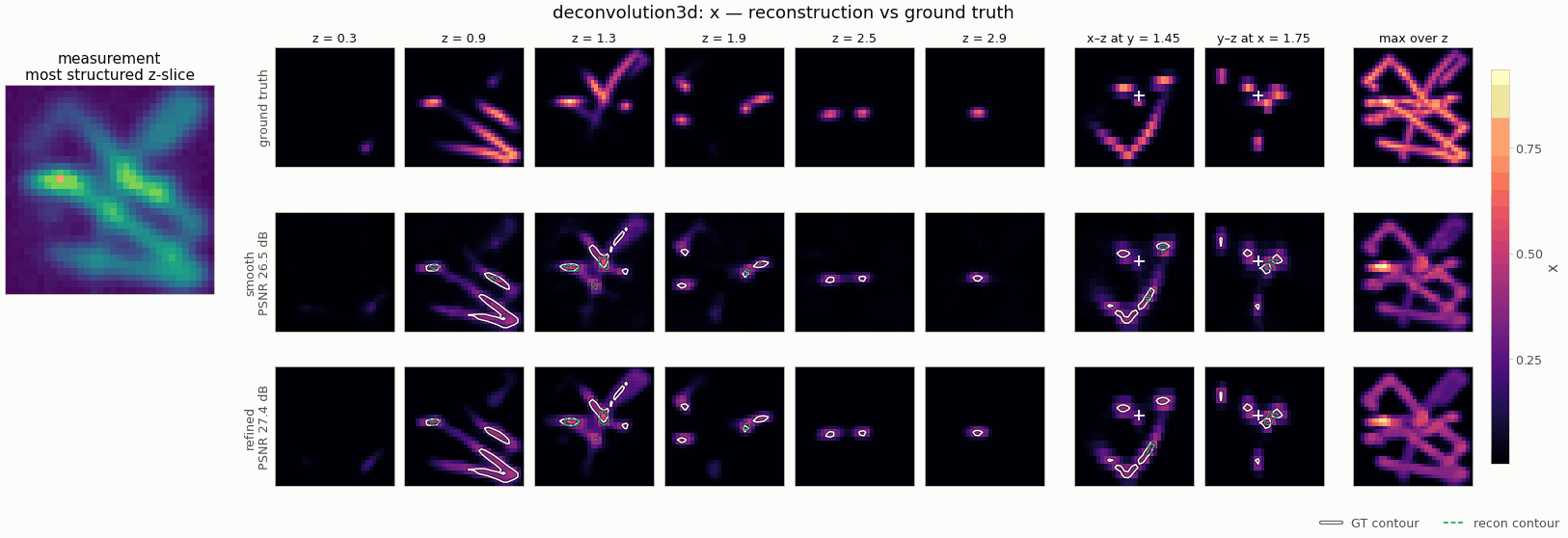
| 3-D deconvolution | fluorophores from a blurred z-stack | 32²×16 · 800 · 12.5 s | PSNR 26.5 dB · refined IoU 0.65 → 0.71 |
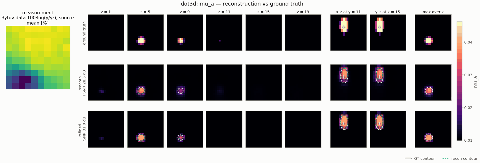
| Diffuse optical tomography | absorption from surface reflectance, 9 sources | 20²×10 · 700 · 17.9 s | PSNR 28.5 dB · refined IoU 0.71 → 0.74 |
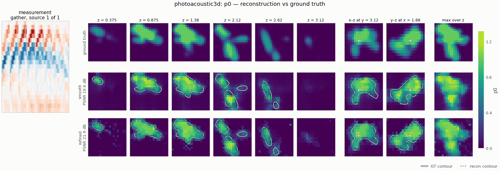
| Photoacoustic tomography | initial pressure from 64 sensor traces | 20²×14 · 400 · 8.4 s | PSNR 19.6 dB · refined IoU 0.73 → 0.80 |
The PSNR of thermal tomography is low because the bulk diffusivity is biased: with the smoke preset's coarse implicit time step the inversion compensates model error by raising α (the model-error floor, see Limitations and caveats). The defect itself is recovered (IoU 0.98).
System by system
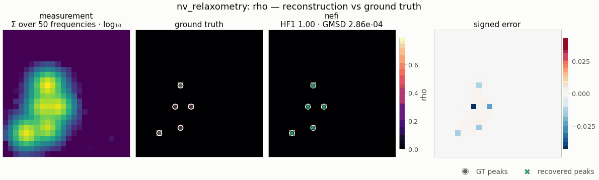
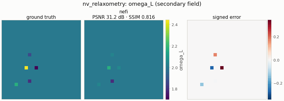
Each figure shows the measurement, the ground truth, the reconstruction (with its metrics) and the signed error; the volumetric systems show depth slices, cross-sections through the anomaly and a projection. The same figures open every instance page.
Optimization in motion
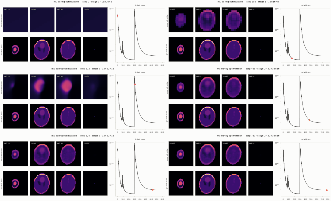
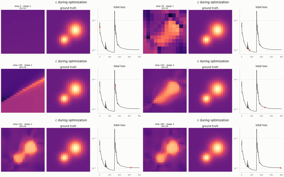
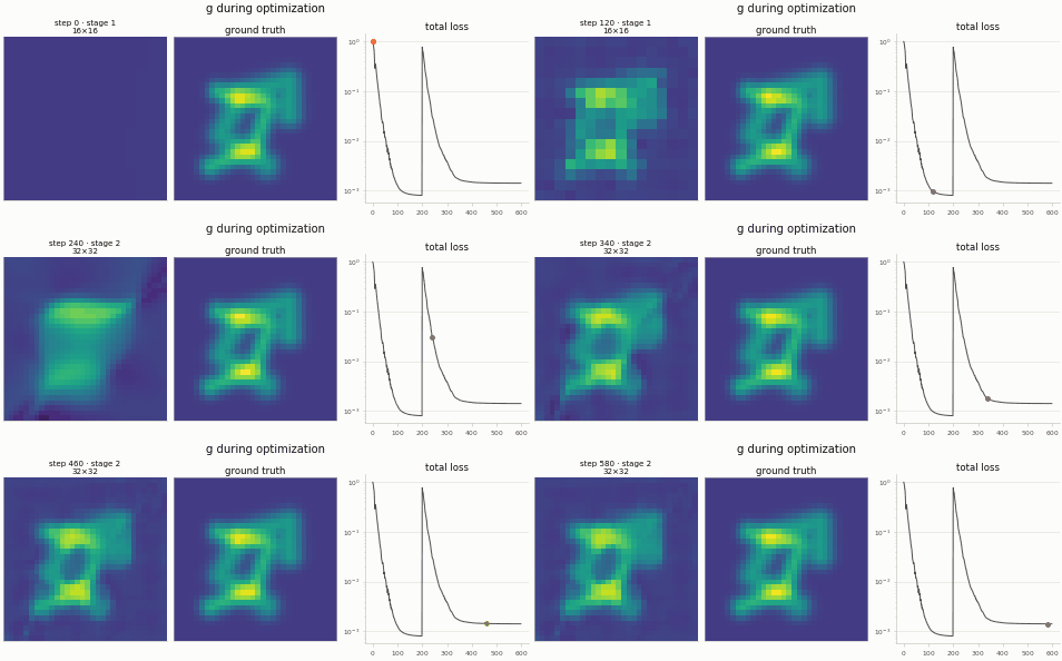
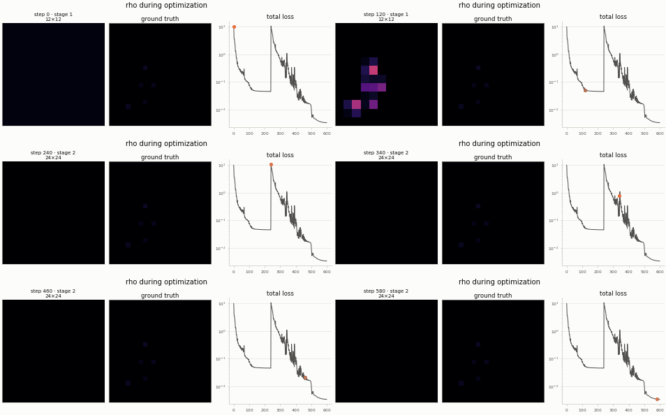
The field during optimization — the coarse stage finds the structure, the fine stage adds detail after the annealed frequency bands reopen (the red dot marks the step on the loss curve).
Reproduce the gallery
python examples/gallery.py --budget 0.2 --out runs/gallery --html    # CPU, about 3 minutes
python examples/gallery.py --budget 1.0 --device cuda --out runs/gallery --html   # full budgets
--html writes a self-contained index.html report with every figure and the interactive
viewers. See Visualization for the figure types and the options.